Chapter 9 Selecting a Preferred Nesting Structure

library(mlogit)

## Loading required package: dfidx

## 
## Attaching package: 'dfidx'

## The following object is masked from 'package:stats':
## 
##     filter

library(tidyverse)

## ── Attaching packages ─────────────────────────────────────── tidyverse 1.3.0 ──

## ✓ ggplot2 3.3.3     ✓ purrr   0.3.4
## ✓ tibble  3.1.1     ✓ dplyr   1.0.5
## ✓ tidyr   1.1.3     ✓ stringr 1.4.0
## ✓ readr   1.4.0     ✓ forcats 0.5.1

## ── Conflicts ────────────────────────────────────────── tidyverse_conflicts() ──
## x dplyr::filter() masks dfidx::filter(), stats::filter()
## x dplyr::lag()    masks stats::lag()

library(modelsummary)
library(haven)
library(knitr)
library(kableExtra)

## 
## Attaching package: 'kableExtra'

## The following object is masked from 'package:dplyr':
## 
##     group_rows

sf_work <- read_rds("data/worktrips.rds")

9.1 Introduction

This chapter re-examines the San Francisco mode choice models estimated in CHAPTER 6 and CHAPTER 7 and evaluates whether the MNL models should be replaced by nested logit models. The final, un-segmented, specifications, Model 17W for work trips and Model 14 S/O for shop/other trips, are taken as the base specifications for estimating nested logit models . Nested models for work trips are examined first, followed by shop/other trips. The chapter concludes with consideration of the policy implications of adopting alternative nesting structures.
Although the number of possible nests for six alternatives is large, the nature of the alternatives allows certain nests to be rejected as implausible. For example, it is unreasonable to suppose that Bike and Transit have substantial unobserved characteristics that lead to correlation in the error terms of their utility functions. For this reason, this chapter considers four plausible nests which are combined in different ways. For Work trips , these are: • Motorized (M) alternatives, comprised of Drive Alone, Shared Ride 2, Shared Ride 3+, and Transit; • Private automobile (P) alternatives, including Drive Alone, Shared Ride 2 and Shared Ride 3+ alternatives; • Shared ride (S) alternatives; and • Non-Motorized (NM) alternatives comprised of Bike and Walk.

Given these four nests or groupings of alternatives and recognizing that Motorized includes both Automobile and Transit alternatives and that Automobile includes Drive Alone and the Shared Ride alternatives, fifteen nest structures as described below. We begin with four single nest models (and, based on the results of these estimations, we explore a selection of more complex structures.

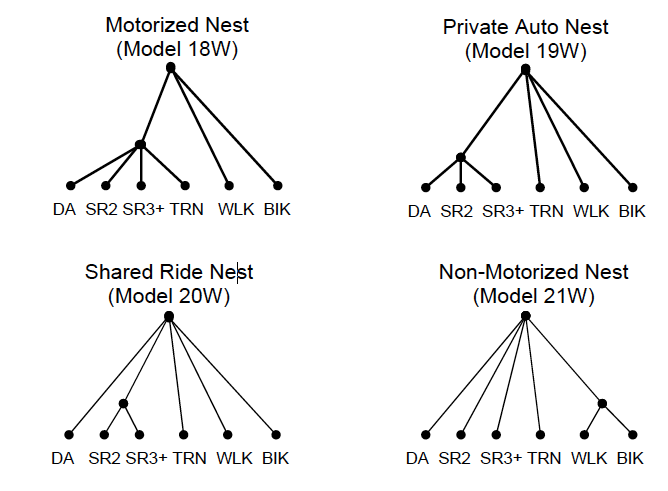
Figure 9.1: Single Nest Models

9.2 Nested Models for Work Trips

The estimation of nested logit models for work trips begins with consideration of the four single nest models mentioned above and illustrated in Figure 9.1. Each of these models obtains improved goodness-of-fit relative to the MNL model (see Table ??). Three of the four models; Models 18W, 20W, 21W; result in acceptable logsum parameters and two of these models (Models 18W and 20W) significantly reject the MNL model at close to the 0.05 level (see the chi-square test and significance in the Table ??. However, the model with the private automobile nest (Model 19W) is rejected because the logsum parameter is greater than one and the model with the non-motorized nest (Model 21W) cannot reject the MNL model at any reasonable level.

work_formula <- chosen ~ I(cost / hhinc) + mot_tvtt + nm_tvtt + movtbyds |  
                 hhinc + vehbywrk + I(wkccbd+wknccbd) + wkempden
m17w <- mlogit(work_formula, data = sf_work)
m18w <- mlogit(work_formula, data = sf_work, 
               nests = list(motorized = c('Drive alone', 'Share ride 2', 
                                          'Share ride 3+', 'Transit'),  
                            other = c('Bike', 'Walk')),
               constPar = c("iv:other" = 1))
m19w <- mlogit(work_formula, data = sf_work, 
               nests = list(privateauto = c('Drive alone', 'Share ride 2', 
                                          'Share ride 3+'),  
                            other = c('Bike', 'Walk', "Transit")),
               constPar = c("iv:other" = 1))
m20w <- mlogit(work_formula, data = sf_work,
               nests = list( shared_ride = c('Share ride 2', 'Share ride 3+'),  
                            other = c('Drive alone',  'Bike','Transit',  'Walk')),
               constPar = c("iv:other" = 1))
m21w <- mlogit(work_formula, data = sf_work,
               nests = list(non_motorized = c('Bike', 'Walk'),  
                            other = c('Drive alone','Share ride 2', 'Share ride 3+', 'Transit')),
               constPar = c("iv:other" = 1))

this_map <- c(
  "I(cost/hhinc)" = "Travel Cost by Income" ,
  "mot_tvtt" = "Motorized Modes Travel Time",
  "nm_tvtt" = "Non-Motorized Modes Travel Time",
  "movtbyds" = "Motorized OVT by Distance",
#"hhinc:Share ride 2", 
#"hhinc:Share ride 3++", 
#"hhinc:Transit", 
#"hhinc:Bike", 
#"hhinc:Walk", 
#"vehbywrk:Share ride 2", 
#"vehbywrk:Share ride 3++", 
#"vehbywrk:Transit", 
#"vehbywrk:Bike", 
#"vehbywrk:Walk", 
#"wknccbd:Share ride 2", 
#"wknccbd:Share ride 3++", 
#"wknccbd:Transit", 
#"wknccbd:Bike", 
#"wknccbd:Walk", 
#"wkempden:Share ride 2", 
#"wkempden:Share ride 3++", 
#"wkempden:Transit", 
#"wkempden:Bike", 
#"wkempden:Walk",
"(Intercept):Share ride 2"   = "Constants Shared ride 2",
"(Intercept):Share ride 3++" = "Constant: Shared ride 3+", 
"(Intercept):Transit"        = "Constant: Transit", 
"(Intercept):Bike"           = "Constant: Bike", 
"(Intercept):Walk"           = "Constant: Walk",
"iv:motorized" = "Motorized Nesting Coefficient",
"iv:privateauto" = "Private Auto Nesting Coefficient",
"iv:shared_ride" = "Shared Ride Nesting Coefficient",
"iv:non_motorized" = "Non-Motorized Nesting Coefficient"
)

single_nest <- list(
  "Model 17W" = m17w,
  "Model 18W" = m18w,
  "Model 19W" = m19w,
  "Model 20W" = m20w,
  "Model 21W" = m21w
  )

modelsummary(single_nest,
             fmt = "%.4f", coef_map = this_map, statistic = "statistic", statistic_vertical = FALSE)

## Warning in sanity_ellipsis(vcov, ...): The `statistic_vertical` argument
## is deprecated and will be ignored. To display uncertainty estimates next to
## your coefficients, use a `glue` string in the `estimate` argument. See `?
## modelsummary`

	Model 17W	Model 18W	Model 19W	Model 20W	Model 21W
Travel Cost by Income	-0.0528	-0.0395	-0.0593	-0.0519	-0.0523
	(-4.9053)	(-4.2108)	(-5.7704)	(-6.3229)	(-6.1333)
Motorized Modes Travel Time	-0.0202	-0.0147	-0.0201	-0.0199	-0.0199
	(-5.2937)	(-3.8350)	(-5.1626)	(-5.3383)	(-5.2238)
Non-Motorized Modes Travel Time	-0.0455	-0.0463	-0.0462	-0.0454	-0.0454
	(-7.8846)	(-7.8793)	(-7.8626)	(-7.7239)	(-7.9588)
Motorized OVT by Distance	-0.1326	-0.1121	-0.1358	-0.1333	-0.1348
	(-6.7530)	(-6.1534)	(-8.1074)	(-8.0397)	(-8.1464)
Constants Shared ride 2	-1.6976	-1.2544	-2.3621	-1.6378	-1.6979
	(-11.9649)	(-5.1759)	(-10.6522)	(-13.1040)	(-12.6106)
Constant: Shared ride 3+	-3.7733	-2.7579	-5.4127	-2.2766	-3.7731
	(-16.0157)	(-5.1891)	(-10.6748)	(-8.8225)	(-15.8012)
Constant: Transit	-0.6930	-0.4163	-0.8374	-0.7012	-0.6896
	(-2.7770)	(-1.9336)	(-3.4063)	(-2.9420)	(-2.8847)
Constant: Bike	-1.6233	-1.3842	-1.7911	-1.6214	-1.4406
	(-3.7840)	(-3.4839)	(-4.6187)	(-4.2150)	(-4.0044)
Constant: Walk	0.0751	0.3337	-0.0882	0.0737	0.0861
	(0.2151)	(0.8824)	(-0.2441)	(0.2071)	(0.2501)
Motorized Nesting Coefficient		0.7269
		(5.4832)
Private Auto Nesting Coefficient			1.4788
			(13.4001)
Shared Ride Nesting Coefficient				0.2994
				(3.0847)
Non-Motorized Nesting Coefficient					0.7673
					(4.1552)
Num.Obs.	5029	5029	5029	5029	5029
AIC	6941.6	6942.0	6929.1	6940.4	6944.3
BIC
Log.Lik.	-3441.782	-3439.980	-3433.532	-3439.198	-3441.156
rho2	0.2914	0.2918	0.2931	0.2919	0.2915
rho20	0.6180	0.6182	0.6190	0.6183	0.6181

tibble(
  model_name = names(single_nest),
  model = single_nest,
) %>%
  mutate(
    loglik = map_dbl(model, logLik),
    lrtest = -2 * (loglik[1] - loglik) ,
    p.value = pchisq(lrtest, 1, lower.tail = FALSE)
  ) %>%
  select(-model) %>%
  kbl(col.names = c("Model", "Log Likelihood", "LR Test", "p-value")) %>% kable_styling()

Model	Log Likelihood	LR Test	p-value
Model 17W	-3441.782	0.000000	1.0000000
Model 18W	-3439.980	3.603876	0.0576450
Model 19W	-3433.532	16.500446	0.0000486
Model 20W	-3439.198	5.168401	0.0230014
Model 21W	-3441.156	1.251722	0.2632239

Next we consider three models with the non-motorized nest in parallel with each of the three other nests (Figure 9.2). In each case, the new models in Table 9-2; Models 22W, 23W and 24W; have better goodness of fit than the corresponding single nest models. Model 23W is rejected because the nest parameter for private automobile is greater than one, as before. Models 22W and 23W both reject the single non-motorized nest (Model 21W) at close to the 0.05 level; however, neither rejects the corresponding Motorized and Shared Ride models (Models 18W and 20W, respectively). In such cases, the analyst can decide to include the non-motorized nest or not, for other than statistical reasons.

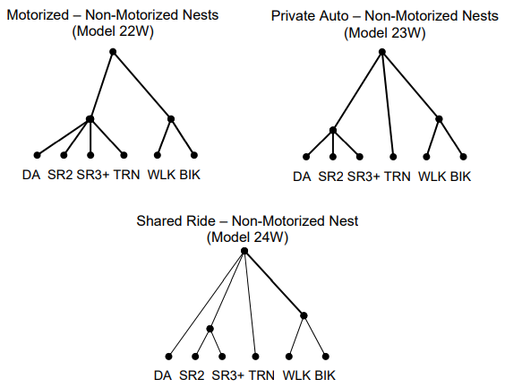
Figure 9.2: Non-Motorized Nest in Parallel with Motorized, Private Automobile and Shared Ride Nests

m22w <- mlogit(work_formula, data = sf_work,
               nests = list(motorized = c('Drive alone', 'Share ride 2', 
                                          'Share ride 3+', 'Transit'),  
                            non_motorized = c('Bike', 'Walk')))
m23w <- mlogit(work_formula, data = sf_work,
               nests = list(auto = c('Drive alone', 'Share ride 2', 'Share ride 3+'),  
                            transit = c("Transit"), non_motorized = c('Bike', 'Walk')),
               constPar = c("iv:transit" = 1))
m24w <- mlogit(work_formula, data = sf_work,
               nests = list(shared = c('Share ride 2', 'Share ride 3+'),  
                            other = c("Drive alone", "Transit"), non_motorized = c('Bike', 'Walk')),
               constPar = c("iv:other" = 1))

parallel_nest <- list(
  "Model 17W" = m17w,
  "Model 22W" = m22w,
  "Model 23W" = m23w,
  "Model 24W" = m24w
  )

modelsummary(parallel_nest,
             fmt = "%.4f", coef_map = this_map, statistic = "statistic", statistic_vertical = FALSE)

## Warning in sanity_ellipsis(vcov, ...): The `statistic_vertical` argument
## is deprecated and will be ignored. To display uncertainty estimates next to
## your coefficients, use a `glue` string in the `estimate` argument. See `?
## modelsummary`

	Model 17W	Model 22W	Model 23W	Model 24W
Travel Cost by Income	-0.0528	-0.0394	-0.0585	-0.0516
	(-4.9053)	(-4.2195)	(-5.6989)	(-6.2406)
Motorized Modes Travel Time	-0.0202	-0.0146	-0.0198	-0.0195
	(-5.2937)	(-3.8326)	(-5.0862)	(-5.2275)
Non-Motorized Modes Travel Time	-0.0455	-0.0463	-0.0460	-0.0446
	(-7.8846)	(-8.1136)	(-8.0568)	(-7.8563)
Motorized OVT by Distance	-0.1326	-0.1138	-0.1384	-0.1344
	(-6.7530)	(-6.2360)	(-8.2700)	(-8.1193)
Constants Shared ride 2	-1.6976	-1.2583	-2.3612	-1.6373
	(-11.9649)	(-5.2194)	(-10.6454)	(-13.0660)
Constant: Shared ride 3+	-3.7733	-2.7657	-5.4110	-2.3204
	(-16.0157)	(-5.2323)	(-10.6689)	(-8.1172)
Constant: Transit	-0.6930	-0.4151	-0.8323	-0.7057
	(-2.7770)	(-1.9268)	(-3.3868)	(-2.9593)
Constant: Bike	-1.6233	-1.2033	-1.6157	-1.4757
	(-3.7840)	(-3.2425)	(-4.4488)	(-4.1092)
Constant: Walk	0.0751	0.3451	-0.0812	0.0657
	(0.2151)	(0.9398)	(-0.2320)	(0.1910)
Motorized Nesting Coefficient		0.7289
		(5.5350)
Non-Motorized Nesting Coefficient		0.7698	0.7652	0.7579
		(4.2012)	(4.1873)	(4.1389)
Num.Obs.	5029	5029	5029	5029
AIC	6941.6	6940.7	6929.8	6941.1
BIC
Log.Lik.	-3441.782	-3439.343	-3432.889	-3438.531
rho2	0.2914	0.2919	0.2932	0.2921
rho20	0.6180	0.6183	0.6190	0.6184

tibble(
  model_name = names(parallel_nest),
  model = parallel_nest,
) %>%
  mutate(
    loglik = map_dbl(model, logLik),
    lrtest = -2 * (loglik[1] - loglik) ,
    p.value = pchisq(lrtest, 1, lower.tail = FALSE)
  ) %>%
  select(-model) %>%
  kbl(col.names = c("Model", "Log Likelihood", "LR Test", "p-value")) %>% kable_styling()

Model	Log Likelihood	LR Test	p-value
Model 17W	-3441.782	0.000000	1.0000000
Model 22W	-3439.343	4.878942	0.0271863
Model 23W	-3432.889	17.785788	0.0000247
Model 24W	-3438.531	6.502062	0.0107749

Another option is to consider ‘hierarchical’ two nest models with Motorized and Private Automobile, Motorized and Shared Ride or Private Automobile and Shared Ride as illustrated in Figure 9.3. Of the three models reported in Table 9-3, only Model 26W, Motorized and Shared Ride, produces an acceptable result. Model 27W is rejected because the private automobile nest coefficient is greater than one, as before. Model 25W is also rejected, despite the fact that the automobile nest parameter is less than one because it is greater than the logsum parameter for the motorized nest which is above it (see Section 8.4). Model 26W, however, represents an attractive model achieving the best goodness-of-fit of any of the models considered, with acceptable logsum parameters. Further, it rejects the MNL model (Model 17W), the Motorized (Model 18W) and the Shared Ride (Model 20W) nest models at roughly the 0.03, 0.07 and 0.06 levels, respectively.

Table 9-4 presents four additional nested model structures for work trips. The first two models extend the nesting structures previously estimated. Model 28W adds the non-motorized nest to Model 26W (see Figure 9.4) with further improved goodness-of-fit, but cannot reject Model 26W at any reasonable level of significance. Model 29W which includes the Motorized, Private Automobile and Shared Ride Nests (see Figure 9.3) is infeasible as it obtains a logsum for the automobile nest that is greater than for the motorized nest, as before. However, Model 29W presents a structure that represents our expectation of the relationship among the motorized modes. Thus, we estimate Model 30W which is identical to Model 29W except that it constrains the automobile nest parameter to 0.75 times the value of the motorized nest parameter. While Model 30W results in a poorer goodness-of-fit than any of the other models including the simple MNL model; it is worth considering because it reflects increased substitution as we move from the Motorized Nest to the Private Automobile Nest to the Shared Ride Nest, as expected. The data does not support this structure (relative to the MNL) but if the analyst or policy makers are convinced it is correct, the use of the relational constraint can produce a model consistent with these assumptions.

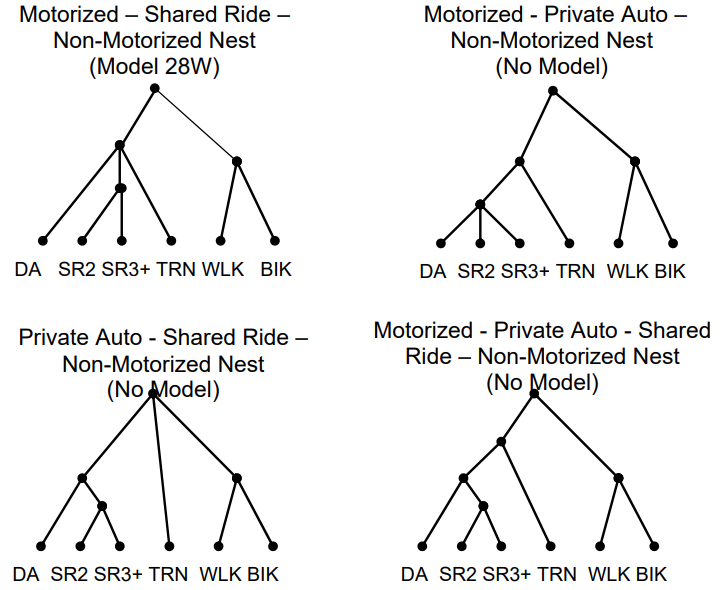
Figure 9.3: Complex Nested Models

The final model, Model 31W, extends Model 30W by adding the Non-Motorized nest to the structure. It therefore has the same issues regarding the constrained nest parameters, but it offers the advantage of including the substitution effects associated with all four nests previously selected. Again, the decision on the acceptance of this model may be based primarily on the judgment of analysts and policy makers.

Based on these results, Models 26W, 28W, 30W and 31W are all potential candidates for a final model. Model 26W is not rejected by any other model and is the simplest structure of this group. Model 28W is slightly better than Model 26W but enough to statistically reject it. Models 30W and 31W have a poorer goodness of fit than Model 26W and 28W, respectively but they incorporate the private automobile intermediate nest. The decision about which of these models to use is largely a matter of judgment. It is possible that other models might also be considered. We further examine Model 26W, because of its simplicity, to demonstrate the differences in direct-elasticity and cross-elasticity between the MNL (17W) model and pairs of alternatives in different parts of the NL tree associated with 26W.

parallel_nest <- list(
  #"Model 17W" = m17w,
  #"Model 26W" = m26w
  )

The structure of the nested logit model (26W) in Figure 9.3 is reproduced here so that each nest can be readily identified. The following table reports the elasticities for the MNL Model 17W and the NL Model 26W.

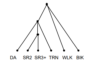
Figure 9.4: Motorized-Shared Ride Nest (Model 26W)

It is apparent from the above table that reduction in the magnitude of the utility parameter for the NL model results in a lower direct and cross elasticity for alternatives that are in neither of the nests depicted in Figure 9.5 than they would have in the corresponding MNL model while alternatives in the lowest and intermediate nests have increased elasticity. The magnitude in of the elasticity increases as alternatives or pairs of alternatives are in lower nests in the tree. Possibly, a better way to think about this is that adoption of the MNL model results in some type of averaged elasticities rather than the distinct elasticities for alternatives in a properly formed NL model.

9.3 Nested Models for Shop / Other Trips

The exploration of nested logit models for shop/other trips follows the same approach as used with work trips, beginning with the consideration of four single nest models depicted in Figure 9.4. For these trips, all four of the single nest structures produce valid models (Table 9-6). Further, Models 15 S/O, 16 S/O and 17 S/O strongly reject the MNL model; however, the non-motorized nest (Model 18 S/O) does not reject the MNL model at any reasonable level of significance.

sf_shopother <- read_rds("data/shopother.rds")
#"Transit", "Share 2", "Share 3+","Drive alone and Share 2/3+", "Share 2/3+","Bike", "Walk", "Drive alone"

#This table has the right idea, though I'm not sure what I can do to fix it or make it more accurate. I also don't know why it isn't showing the other constants...
SO_formula <- chosen ~ totcost + tvtt  + I(totcost/log(income)) + ovttdist |  
                 income + veh_wkr + ave_dens
m14SO <- mlogit(SO_formula, data = sf_shopother)
m15SO <- mlogit(SO_formula, data = sf_shopother,
               nests = list(motorized = c('Drive alone', 'Drive alone and Share 2/3+', 'Share 2/3+','Transit',
                                          'Share 2','Share 3+'),  
                             non_motorized = c('Bike', 'Walk')),
               constPar = c("iv:non_motorized" = 1))
m16SO <- mlogit(SO_formula, data = sf_shopother,
               nests = list(private_auto = c('Drive alone', 'Drive alone and Share 2/3+', 'Share 2/3+',
                                          'Share 2','Share 3+'), 
                            other = c('Transit', 'Bike', 'Walk')),
               constPar = c("iv:other" = 1))
m17SO <- mlogit(SO_formula, data = sf_shopother,
               nests = list(shared = c('Share 2/3+','Transit',
                                          'Share 2','Share 3+'),  
                            other = c("Drive alone", "Transit",'Bike', 'Walk','Drive alone and Share 2/3+')),
               constPar = c("iv:other" = 1))
m18SO <- mlogit(SO_formula, data = sf_shopother,
               nests = list(other = c('Drive alone', 'Drive alone and Share 2/3+', 'Share 2/3+','Transit',
                                          'Share 2','Share 3+'), 
                            non_motorized = c('Bike', 'Walk')),
               constPar = c("iv:other" = 1))

parallel_nests <- list(
  "Model 14SO" = m14SO,
  "Model 15SO" = m15SO,
  "Model 16SO" = m16SO,
  "Model 17SO" = m17SO,
  "Model 18SO" = m18SO
  )

modelsummary(parallel_nests,
             fmt = "%.4f", coef_map = this_map, statistic = "statistic", statistic_vertical = FALSE)

## Warning in sanity_ellipsis(vcov, ...): The `statistic_vertical` argument
## is deprecated and will be ignored. To display uncertainty estimates next to
## your coefficients, use a `glue` string in the `estimate` argument. See `?
## modelsummary`

	Model 14SO	Model 15SO	Model 16SO	Model 17SO	Model 18SO
Constant: Bike	-7.7607	-7.0614	-7.0490	-7.4427	-6.6157
	(-9.6801)	(-5.0223)	(-7.7275)	(-7.6222)	(-8.2790)
Constant: Walk	-3.5504	-2.7343	-2.9676	-3.1170	-3.6332
	(-5.3377)	(-2.0550)	(-3.9906)	(-3.6214)	(-5.7231)
Motorized Nesting Coefficient		2.7352
		(3.6668)
Non-Motorized Nesting Coefficient					0.5724
					(4.4713)
Num.Obs.	3157	3157	3157	3157	3157
AIC	9581.8	9570.9	9567.4	9576.5	9581.3
BIC
Log.Lik.	-4758.915	-4751.453	-4749.720	-4754.236	-4756.626
rho2	0.0668	0.0683	0.0686	0.0677	0.0673
rho20	0.2751	0.2762	0.2765	0.2758	0.2754

Despite the marginal significance of the non-motorized nest, the possible two parallel nest models including non-motorized and one other nest, were estimated and are reported in Table 9-7. All three specifications result in valid models with improved goodness-of-fit over the MNL and the single nest NM model (Model 18 S/O) but Models 19 S/O, 20 S/O and 21 S/O do not reject the corresponding Motorized (Model 15 S/O), Private Automobile (Model 16 S/O) and Shared Ride (Model 17 S/O) nest models, which are restricted forms of these models, at a high level of confidence.
It is important to note that a variety of different initial parameters were required to find the solution for Model 20 S/O reported here. The selection of different starting values for the model parameters, especially the nest parameter(s) may lead to convergence at different values in or out of the acceptable range as discussed in CHAPTER 10.

As in the case of work trips, hierarchical two-nest models, depicted in Figure 9.2, are considered next, Table 9-8. Model 22 S/O obtains a satisfactory parameter for the automobile logsum but the motorized logsum is not significantly different from one and the model does not reject the single nest Private Automobile structure (Model 16 S/O). However, Models 23 S/O (with shared ride under the motorized nest) and 24 S/O (with shared ride under the automobile nest) provide excellent results. The similarity interpretation of these nests is reasonable and both models strongly reject the MNL model and the constrained single nest models reported in Table 9-7.

m22SO <- mlogit(work_formula, data = sf_work,
               nests = list(motorized = c('Drive alone', 'Share ride 2', 
                                          'Share ride 3+', 'Transit'),  
                            non_motorized = c('Bike', 'Walk')))
m23SO <- mlogit(work_formula, data = sf_work,
               nests = list(auto = c('Drive alone', 'Share ride 2', 'Share ride 3+'),  
                            transit = c("Transit"), non_motorized = c('Bike', 'Walk')),
               constPar = c("iv:transit" = 1))
m24SO <- mlogit(work_formula, data = sf_work,
               nests = list(shared = c('Share ride 2', 'Share ride 3+'),  
                            other = c("Drive alone", "Transit"), non_motorized = c('Bike', 'Walk')),
               constPar = c("iv:other" = 1))



parallel_nest <- list(
  #"Model 14SO" = m14SO,
  "Model 22SO" = m22SO,
  "Model 23SO" = m23SO,
  "Model 24SO" = m24SO
  )

modelsummary(parallel_nest)

	Model 22SO	Model 23SO	Model 24SO
(Intercept) × Share ride 2	-1.258	-2.361	-1.637
	(0.241)	(0.222)	(0.125)
(Intercept) × Share ride 3++	-2.766	-5.411	-2.320
	(0.529)	(0.507)	(0.286)
(Intercept) × Transit	-0.415	-0.832	-0.706
	(0.215)	(0.246)	(0.238)
(Intercept) × Bike	-1.203	-1.616	-1.476
	(0.371)	(0.363)	(0.359)
(Intercept) × Walk	0.345	-0.081	0.066
	(0.367)	(0.350)	(0.344)
I(cost/hhinc)	-0.039	-0.059	-0.052
	(0.009)	(0.010)	(0.008)
mot_tvtt	-0.015	-0.020	-0.020
	(0.004)	(0.004)	(0.004)
nm_tvtt	-0.046	-0.046	-0.045
	(0.006)	(0.006)	(0.006)
movtbyds	-0.114	-0.138	-0.134
	(0.018)	(0.017)	(0.017)
hhinc × Share ride 2	0.000	-0.002	0.000
	(0.001)	(0.002)	(0.001)
hhinc × Share ride 3++	0.002	0.001	0.001
	(0.002)	(0.003)	(0.002)
hhinc × Transit	-0.004	-0.005	-0.005
	(0.002)	(0.002)	(0.002)
hhinc × Bike	-0.010	-0.008	-0.009
	(0.004)	(0.004)	(0.004)
hhinc × Walk	-0.006	-0.005	-0.006
	(0.003)	(0.003)	(0.003)
vehbywrk × Share ride 2	-0.271	-0.605	-0.341
	(0.071)	(0.115)	(0.060)
vehbywrk × Share ride 3++	-0.107	-0.257	-0.278
	(0.082)	(0.164)	(0.070)
vehbywrk × Transit	-0.705	-0.862	-0.948
	(0.145)	(0.110)	(0.104)
vehbywrk × Bike	-0.736	-0.599	-0.699
	(0.197)	(0.197)	(0.195)
vehbywrk × Walk	-0.764	-0.612	-0.713
	(0.139)	(0.141)	(0.139)
I(wkccbd + wknccbd) × Share ride 2	0.183	0.388	0.388
	(0.097)	(0.181)	(0.113)
I(wkccbd + wknccbd) × Share ride 3++	0.800	1.641	0.626
	(0.203)	(0.317)	(0.142)
I(wkccbd + wknccbd) × Transit	0.920	1.364	1.324
	(0.220)	(0.185)	(0.179)
I(wkccbd + wknccbd) × Bike	0.403	0.443	0.443
	(0.328)	(0.333)	(0.329)
I(wkccbd + wknccbd) × Walk	0.107	0.117	0.105
	(0.235)	(0.240)	(0.238)
wkempden × Share ride 2	0.001	0.003	0.002
	(0.000)	(0.001)	(0.000)
wkempden × Share ride 3++	0.002	0.004	0.002
	(0.000)	(0.001)	(0.000)
wkempden × Transit	0.002	0.004	0.003
	(0.000)	(0.000)	(0.000)
wkempden × Bike	0.002	0.003	0.002
	(0.001)	(0.001)	(0.001)
wkempden × Walk	0.002	0.003	0.003
	(0.001)	(0.001)	(0.001)
iv × motorized	0.729
	(0.132)
iv × non_motorized	0.770	0.765	0.758
	(0.183)	(0.183)	(0.183)
iv × auto		1.479
		(0.110)
iv × shared			0.320
			(0.112)
Num.Obs.	5029	5029	5029
AIC	6940.7	6929.8	6941.1
BIC
Log.Lik.	-3439.343	-3432.889	-3438.531
rho2	0.292	0.293	0.292
rho20	0.618	0.619	0.618

Unlike the case of the home-based work models, the home-based shop/other data set supports complex nested models which combine the hierarchical and parallel nests to capture the different substitutability between several groups of alternatives. Models 25 S/O and 26 S/O improve goodness-of-fit over both the best hierarchical (Model 24 S/O) and parallel (Model 20 S/O) two-nest models. These more complex models can reject all of the single nest models at the .05 level or higher, but cannot reject the best two-nest models at a high level of confidence. Even so, they may still be preferred for their potentially more realistic representation of trade-offs between pairs of alternatives. The same rationale could be applied between the two models, as Model 26 S/O cannot reject 25 S/O, either, but allows for greater substitutability between the non-motorized modes (for which the statistical evidence is moderately significant). The nesting coefficient for the motorized nest is not particularly significant in either model, but it can be retained given the reasonableness of its value.

9.4 Practical Issues and Implications

A large number of nested logit structures can be proposed for any context in which the number of alternatives is not very small. As seen, even in the case of four alternatives, there are 25 possible nest structures and this number increases to 235 for five alternatives and beyond 2000 for six or more alternatives. Since searching across this many nest structures is generally infeasible, it is the responsibility of the analyst to propose a subset of these structures for primary consideration or, alternatively, to eliminate a subset of such structures from consideration. At the same time, it is desirable for the analyst to remain open to other possible structures that may be suggested by others who have familiarity with the behavior under study. It is not uncommon for some or all of the proposed structures to be infeasible due to obtaining an estimated logsum or nesting parameter that is greater than one or greater than the parameter in a higher level nest. It is a matter of judgment whether to eliminate the proposed structure based on the estimation results or to constrain selected nest parameters to fixed values or to relative values that ensure that the structure is consistent with utility maximization. This ‘imposition’ of a fixed value or other constraints on nest parameters requires careful judgment, discussion with other modeling and policy analysts and open reporting so that potential users of the model are aware of the basis for the proposed model. An important part of the decision process is the differential interpretation associated with any nested logit model relative to the multinomial logit model or other nested logit models. The central element of such interpretation is the way in which a change in any of the characteristics of an alternative affects the probability of that alternative and each other alternative being chosen. This is the essential element of competition/substitution between pairs of alternatives and may dramatically influence the predicted impact of selected policy changes.