Chapter 4 The Multinomial Logit Model

library(tidyverse)

## ── Attaching packages ─────────────────────────────────────── tidyverse 1.3.0 ──

## ✓ ggplot2 3.3.3     ✓ purrr   0.3.4
## ✓ tibble  3.1.1     ✓ dplyr   1.0.5
## ✓ tidyr   1.1.3     ✓ stringr 1.4.0
## ✓ readr   1.4.0     ✓ forcats 0.5.1

## ── Conflicts ────────────────────────────────────────── tidyverse_conflicts() ──
## x dplyr::filter() masks stats::filter()
## x dplyr::lag()    masks stats::lag()

library(kableExtra)

## 
## Attaching package: 'kableExtra'

## The following object is masked from 'package:dplyr':
## 
##     group_rows

#' Create a tibble object that evaluates the named expressions passed
#' in as utility equation.
utility_table <- function(expressions){
  top <- tibble(
    Alternative = names(expressions),
    Expression = expressions 
  ) %>%
    rowwise() %>%
    mutate(
      Value = eval(parse(text = Expression)),
      Exponent = exp(Value) 
    ) %>%
    ungroup() %>%
    mutate( Probability = Exponent / sum(Exponent) )
  
  bottom <- tibble(
    Alternative = "Total",
    Expression = "",
    Value = NA,
    Exponent = sum(top$Exponent),
    Probability = sum(top$Probability)
  )
  
  bind_rows(top, bottom)
}

4.1 Overview Description and Functional Form

The mathematical form of a discrete choice model is determined by the assumptions made regarding the error components of the utility function for each alternative as described in section 3.5. The specific assumptions that lead to the Multinomial Logit Model are (1) the error components are extreme-value (or Gumbel) distributed, (2) the error components are identically and independently distributed across alternatives, and (3) the error components are identically and independently distributed across observations/individuals. We discuss each of these assumptions below.

The most common assumption for error distributions in the statistical and modeling literature is that errors are distributed normally. There are good theoretical and practical reasons for using the normal distribution for many modeling applications. However, in the case of choice models the normal distribution assumption for error terms leads to the Multinomial Probit Model (MNP) which has some properties that make it difficult to use in choice analysis.¹ The Gumbel distribution is selected because it has computational advantages in a context where maximization is important, closely approximates the normal distribution (see Figure 4.1 and Figure 4.2) and produces a closed-form² probabilistic choice model.

pdf <- tibble(
  x = seq(-5, 5, by = 0.01),
  Normal = dnorm(x, sd = sqrt(pi^2/6)),
  Gumbel = exp(-x) * exp(-exp(-x))
) 

ggplot(pdf %>% gather(key = "Distribution", value = "Probability", -x),
       aes(x = x, y = Probability, color = Distribution)) +
  geom_line() + 
  theme_bw()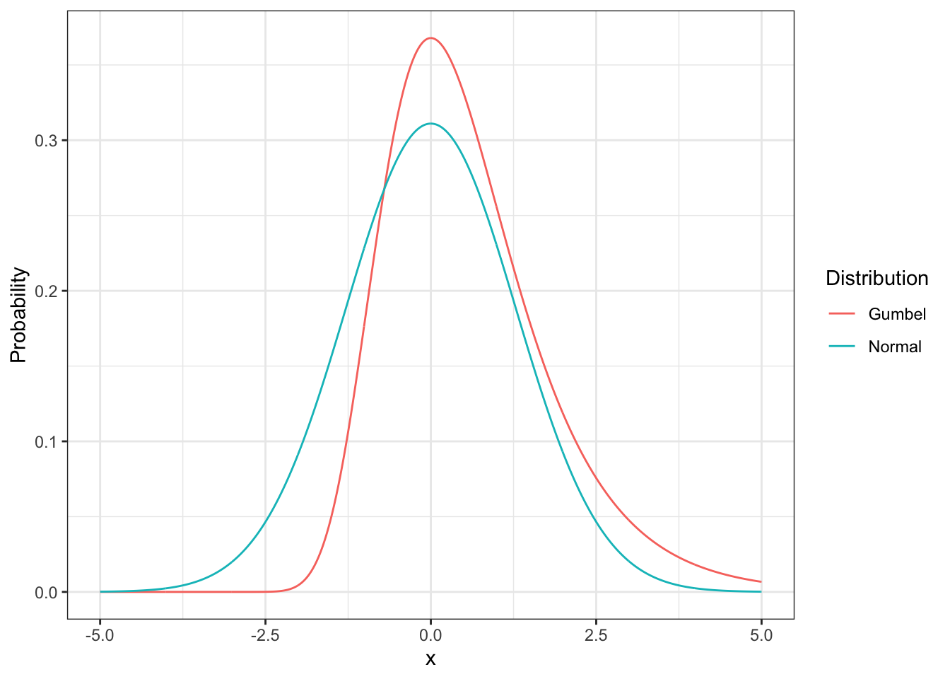

Figure 4.1: Probability density function for normal and Gumbel distributions.

cdf <- tibble(
  x = seq(-4, 5, by = 0.01),
  Normal = pnorm(x, sd = sqrt(pi^2 / 6)),
  Gumbel = exp(-exp(-x))
) 

ggplot(cdf %>% gather(key = "Distribution", value = "Probability", -x),
       aes(x = x, y = Probability, color = Distribution)) +
  geom_line() + 
  theme_bw()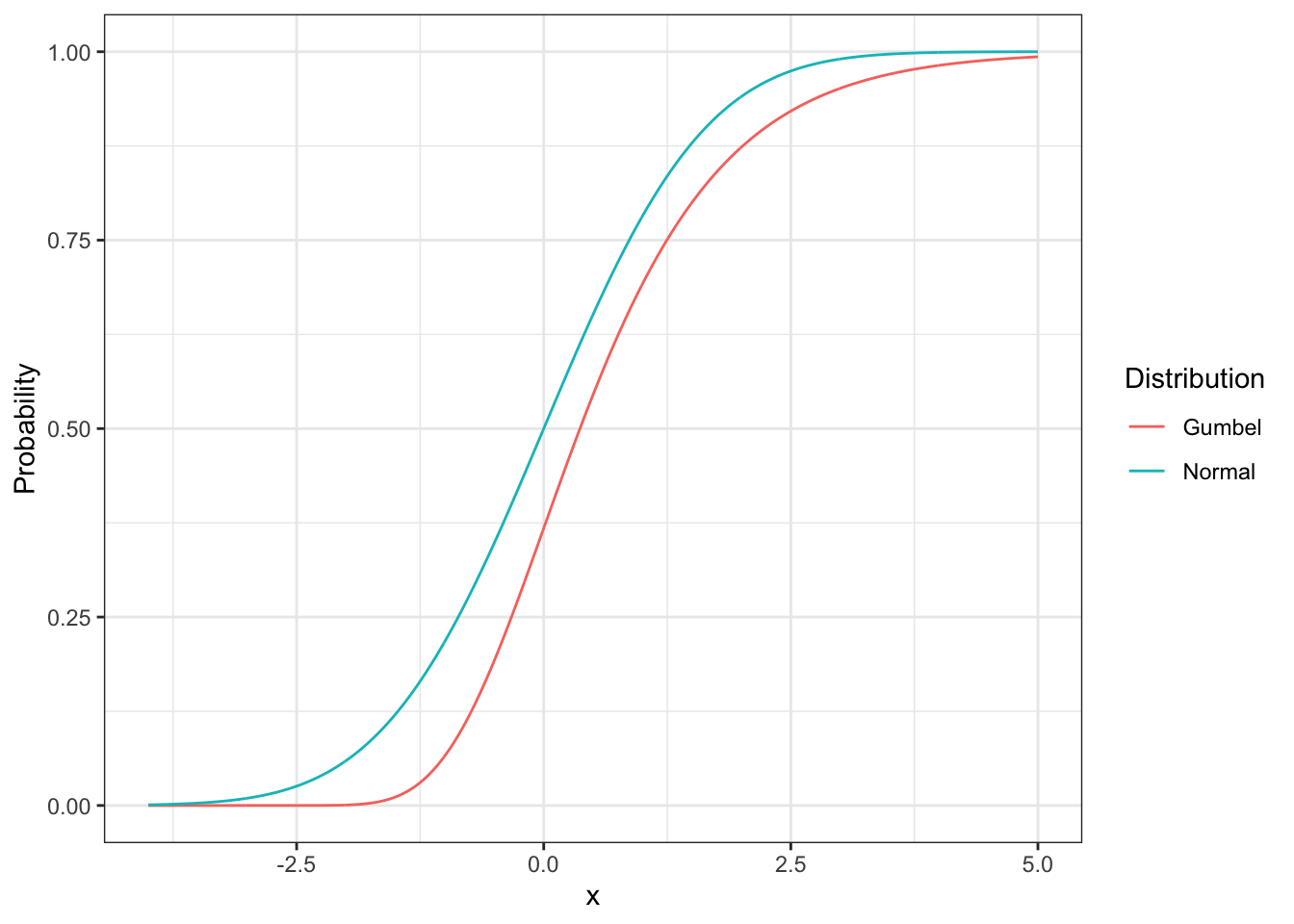

Figure 4.2: Cumulative density function for normal and Gumbel distributions.

The Gumbel has the following cumulative distribution and probability density functions:

\[\begin{equation} F(\epsilon) = e^{e^{-\mu(\epsilon-\eta)}} \tag{4.1} \end{equation}\]

\[\begin{equation} f(\epsilon) = \mu e^{-\mu(\epsilon-\eta)} \times e^{e^{-\mu(\epsilon-\eta)}} \tag{4.2} \end{equation}\]

where

• \(\mu\) is the scale parameter which determines the variance of the distribution and
• \(\eta\) is the location (mode) parameter.

The mean and variance of the distribution are:

\[\begin{equation} Mean = \eta + \frac{0.577}{\mu} \tag{4.3} \end{equation}\]

\[\begin{equation} Variance = \frac{\pi^2}{6\mu^2} \tag{4.4} \end{equation}\]

The second and third assumptions state the location and variance of the distribution just as \(\mu\) and \(\sigma^2\) indicate the location and variance of the normal distribution. We will return to the discussion of the independence between/among alternatives in CHAPTER 8.

The three assumptions, taken together, lead to the mathematical structure known as the Multinomial Logit Model (MNL), which gives the choice probabilities of each alternative as a function of the systematic portion of the utility of all the alternatives. The general expression for the probability of choosing an alternative ‘i’ (i = 1,2,.., J) from a set of J alternatives is:

\[\begin{equation} Pr(i) = \frac{\exp(V_i)}{\sum_{j=1}^{J}\exp(V_j)} \tag{4.5} \end{equation}\]

Where

• \(Pr(i)\) is the probability of the decision-make choosing alternative i and
• \(V_j\) is the systematic component of the utility of alternative j.

The exponential function is described in Figure 4.3 which shows the relationship between \(\exp(V_i)\) and \(V_i\). Note that \(\exp(V_i)\) is always positive and increases monotonically with \(V_i\).

tibble( x = seq(-3,3,.1), y = exp(x)) %>%
  ggplot(aes(x = x, y = y)) + 
  geom_line() + 
  xlab(bquote(V[i])) + 
  ylab(bquote(exp(V[i]))) +
  theme_bw()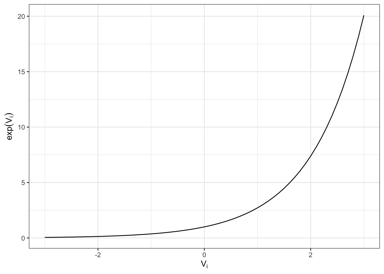

Figure 4.3: Relationship Between \(V_i\) and \(\exp(V_i)\)

The multinomial logit (MNL) model has several important properties. We illustrate these for a case in which the decision maker has three available alternatives: Drive Alone (DA), Shared Ride (SR), and TRansit (TR). The probabilities of each alternative are given by modifying equation 4.5 for each alternative to obtain:

\[\begin{equation} Pr(DA) = \frac{\exp(V_{DA})}{\exp(V_{DA}) + \exp(V_{SR}) + \exp(V_{TR})} \tag{4.6} \end{equation}\]

\[\begin{equation} Pr(SR) = \frac{\exp(V_{SR})}{\exp(V_{DA}) + \exp(V_{SR}) + \exp(V_{TR})} \tag{4.7} \end{equation}\]

\[\begin{equation} Pr(TR) = \frac{\exp(V_{TR})}{\exp(V_{DA}) + \exp(V_{SR}) + \exp(V_{TR})} \tag{4.8} \end{equation}\]

where \(Pr(DA)\), \(Pr(SR)\), and \(Pr(TR)\) are the probabilities of the decision-maker choosing drive alone, shared ride and transit, respectively, and \(V_{DA}\), \(V_{SR}\) and \(V_{TR}\) are the systematic components of the utility for drive alone, shared ride, and transit alternatives, respectively. It is common to replace these three equations by a single general equation to represent the probability of any alternative and to simplify the equation by replacing the explicit summation in the denominator by the summation over alternatives as:

\[\begin{equation} Pr(i) = \frac{\exp(V_{i})}{\exp(V_{DA}) + \exp(V_{SR}) + \exp(V_{TR})} \tag{4.9} \end{equation}\]

\[\begin{equation} Pr(i) = \frac{\exp(V_{i})}{\sum_{j=DA,SR,TR}\exp(V_j)} \tag{4.10} \end{equation}\]

where i indicates the alternative for which the probability is being computed.

This formulation implies that the probability of choosing an alternative increases monotonically with an increase in the systematic utility of that alternative and decreases with increases in the systematic utility of each of the other alternatives. This is illustrated in Table 4.1 showing the probability of DA as a function of its own utility (with the utilities of other alternatives held constant) and in Table ?? as a function of the utility of other alternatives with its own utility fixed.

tibble(
  case = 1:5,
  vda = c(-3.0, -1.5, 0.0, 1.5, 3.0),
  vsr = -1.5,
  vtr = -0.5
) %>%
  mutate(
    p = exp(vda) / (exp(vda) + exp(vsr) + exp(vtr))
  ) %>%
  kableExtra::kbl(  
    caption = "Probability Values for Drive Alone as a Function of Drive Alone Utility (Shared Ride and Transit Utilities held constant)", 
    col.names = c("$Case$", "$V_{DA}$", "$V_{SR}$", "$V_{TR}$", "$Pr(DA)$")) %>%
  kableExtra::kable_styling()

Table 4.1: Probability Values for Drive Alone as a Function of Drive Alone Utility (Shared Ride and Transit Utilities held constant)

\(Case\)	\(V_{DA}\)	\(V_{SR}\)	\(V_{TR}\)	\(Pr(DA)\)
1	-3.0	-1.5	-0.5	0.0566117
2	-1.5	-1.5	-0.5	0.2119416
3	0.0	-1.5	-0.5	0.5465494
4	1.5	-1.5	-0.5	0.8437947
5	3.0	-1.5	-0.5	0.9603322

tibble(
  case = 6:11,
  vda = 0.0,
  vsr = c(-1.5, -1.5, -1.5, -0.5, -0.5, -0.5),
  vtr = c(-1.5, -1.0, -0.5, -1.5, -1.0, -0.5)
) %>%
  mutate(
    p = exp(vda) / (exp(vda) + exp(vsr) + exp(vtr))
  ) %>%
  kableExtra::kbl(
    caption = "Probability Values for Drive Alone as a Function of Shared Ride and Transit Utilties", 
    col.names = c("$Case$", "$V_{DA}$", "$V_{SR}$", "$V_{TR}$", "$Pr(DA)$")) %>%
  kableExtra::kable_styling()

Table 4.2: Probability Values for Drive Alone as a Function of Shared Ride and Transit Utilties

\(Case\)	\(V_{DA}\)	\(V_{SR}\)	\(V_{TR}\)	\(Pr(DA)\)
6	0	-1.5	-1.5	0.6914385
7	0	-1.5	-1.0	0.6285317
8	0	-1.5	-0.5	0.5465494
9	0	-0.5	-1.5	0.5465494
10	0	-0.5	-1.0	0.5064804
11	0	-0.5	-0.5	0.4518628

We use this three-alternative example to illustrate three important properties of the MNL: (1) its sigmoid or S shape, (2) dependence of the alternative choice probabilities on the differences in the systematic utility and (3) independence of the ratio of the choice probabilities of any pair of alternatives from the attributes and availability of other alternatives.

4.1.1 The Sigmoid or S shape of Multinomial Logit Probabilities

The S shape of the MNL probabilities is illustrated in Figure ?? where the probability of choosing Drive Alone is shown as a function of its own utility, with the utilities of the other alternatives held constant. The S-shape limits the probability range between zero when the utility of DA is very low, relative to other alternatives, and one when the utility of DA is very high, relative to other alternatives. This function has very gradual slope at extreme values of DA utility, relative to the other alternatives, and is much steeper when its utility reaches a value such that its choice probability is close to one-half. This implies that if the representative utility of one alternative is very low or very high, compared with the others, a small increase in the utility of this alternative will not substantially affect its probability of being chosen. The point at which an increase in the representative utility of an alternative has the greatest effect on its probability of being chosen (i.e., the point of maximum slope along the curve) is when its representative utility is equivalent to the combined utility of the other alternatives. When this is true, a small increase in the utility of one alternative can ‘tip the balance’ and induce a large increase in the probability of the alternative being chosen (Train, 1993).

#' Function to compute mnl probabilities
#' @param vi utility of target alternative
#' @param ... utilities of other alternatives
mnl_prob <- function(vi, ...){
  vj <- c(...)
  exp(vi) / sum(exp(vj))
}

u <- tibble(
  v_da = seq(-3, 3, by = 0.01),
  v_tr = 0, v_walk = -0.5
) %>% 
  rowwise() %>%
  mutate(
    drive   = mnl_prob(v_da,   v_da, v_tr, v_walk),
    transit = mnl_prob(v_tr,   v_da, v_tr, v_walk),
    walk    = mnl_prob(v_walk, v_da, v_tr, v_walk)
  )

ggplot(u %>% gather(Mode, Probability, drive, transit, walk), 
       aes(x = v_da, y = Probability, color = Mode)) + 
  geom_line() +
  xlab("Utility of Drive") + 
  theme_bw()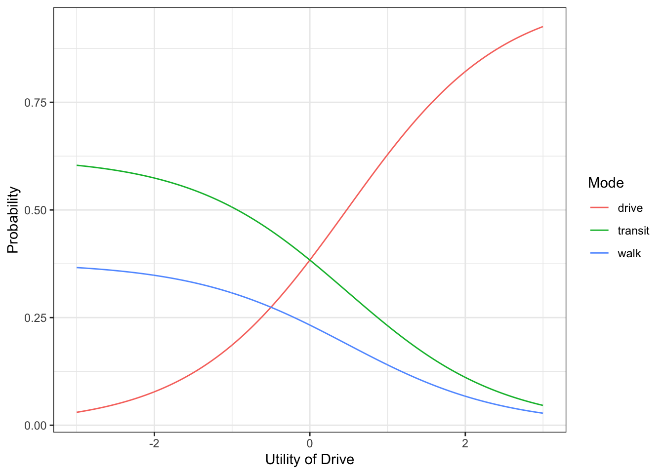

Figure 4.4: Probability of choosing alternatives while holding other utilities constant, \(V_{transit} = 0, V_{walk} = -0.5\)

4.1.2 The Equivalent Differences Property

A fundamental property of the multinomial logit and other choice models is that the choice probabilities of the alternatives depend only on the differences in the systematic utilities of different alternatives and not their actual values. This can be illustrated in two ways. First, we show that the choice probability equations are unchanged if the same incremental value, say \(\Delta V\), is added to the utility of each alternative. The original probabilities for the three alternatives in the example are given by:

\[\begin{equation} Pr(i) = \frac{\exp(V_{i})}{\exp(V_{DA}) + \exp(V_{SR}) + \exp(V_{TR})} \tag{4.11} \end{equation}\]

where i is the alternative for which the probabilities are being computed.

Adding \(\Delta V\) to the systematic components of \(V_{DA}\), \(V_{SR}\) and \(V_{TR}\) gives³:

\[\begin{align*} Pr(i)&= \frac{\exp(V_i + {\Delta V })} {\exp(V_{DA}+{\Delta V }) + \exp(V_{SR}+{\Delta V }) + \exp(V_{TR}+{\Delta V })} \\ &= \frac{\exp(V_i) \times \exp({\Delta V })} {\exp(V_{DA}) \times \exp({\Delta V }) + \exp(V_{SR}) \times \exp({\Delta V }) + \exp(V_{TR}) \times \exp({\Delta V })} \\ &= \frac{\exp(V_i) \times \exp({\Delta V })}{[\exp(V_{DA}) + \exp(V_{SR}) + \exp(V_{TR})] \times \exp({\Delta V })} \\ &= \frac{\exp(V_i)}{[\exp(V_{DA}) + \exp(V_{SR}) + \exp(V_{TR})]} \tag{4.12} \end{align*}\]

which is the same probability as before \(\Delta V\) was added to each of the utilities. This result applies to any value of \(\Delta V\). We also illustrate this property through use of a numerical example for the three alternative choice problem used earlier. The following equations represent the case when the utility values for Drive Alone, Shared Ride and Transit equal 0.5, 1.5 and 3.0, respectively:

\[\begin{equation} Pr(DA) = \frac {\exp(-0.5)}{\exp(-0.5) + \exp(-1.5) + \exp(-3.0)} = 0.690 \tag{4.13} \end{equation}\]

\[\begin{equation} Pr(SR) = \frac {\exp(-1.5)}{\exp(-0.5) + \exp(-1.5) + \exp(-3.0)} = 0.254 \tag{4.14} \end{equation}\]

\[\begin{equation} Pr(TR) = \frac {\exp(-3.0)}{\exp(-0.5) + \exp(-1.5) + \exp(-3.0)} = 0.057 \tag{4.15} \end{equation}\]

Similarly, if the utility of each alternative is increased by one, the probabilities are:

\[\begin{equation} Pr(DA) = \frac {\exp(0.5)}{\exp(0.5) + \exp(-0.5) + \exp(-2.0)} = 0.690 \tag{4.16} \end{equation}\]

\[\begin{equation} Pr(SR) = \frac {\exp(-0.5)}{\exp(0.5) + \exp(-0.5) + \exp(-2.0)} = 0.254 \tag{4.17} \end{equation}\]

\[\begin{equation} Pr(TR) = \frac {\exp(-2.0)}{\exp(0.5) + \exp(-0.5) + \exp(-2.0)} = 0.057 \tag{4.18} \end{equation}\]

As expected, the choice probabilities are identical to those obtained before the addition of the constant utility to each mode. The calculations supporting this comparison are shown in Table 4.3 and Table 4.4. Table 4.3 shows the computation of the choice probabilities based on the initial set of modal utilities and Table 4.4 shows the same computation after each of the utilities is increased by one.⁴

Table 4.3: Numerical Example Illustrating Equivalent Difference Property: Probability of Each Alternative Before Adding Delta

	Utility
Alternative	Expression	Value	Exponent	Probability
Drive Alone	-0.50	-0.5	0.6065307	0.6896721
Shared Ride	-1.50	-1.5	0.2231302	0.2537162
Transit	-3.00	-3.0	0.0497871	0.0566117
Total		NA	0.8794479	1.0000000

where the sum of the exponent variable is equal to 0.879.

Table 4.4: Numerical Example Illustrating Equivalent Difference Property: Probability of Each Alternative After Adding Delta (=1.0)

	Utility
Alternative	Expression	Value	Exponent	Probability
Drive Alone	-0.50 + 1.00	0.5	1.6487213	0.6896721
Shared Ride	-1.50 + 1.00	-0.5	0.6065307	0.2537162
Transit	-3.00 + 1.00	-2.0	0.1353353	0.0566117
Total		NA	2.3905872	1.0000000

Where the sum of the exponent variable is equal to 2.391

The expression for the probability equation of the logit model (equation 4.9) can also be presented in a different form which makes the equivalent difference property more apparent. For the drive alone alternative, this expression can be obtained by multiplying the numerator and denominator of the standard probability expression by (-VDA) as shown in the following equations.

\[\begin{equation} \begin{split} Pr(DA) &= \frac{\exp(V_{DA})}{\exp(V_{DA}) + \exp(V_{SR}) + \exp(V_{TR})} \times \frac {\exp(-V_{DA})}{\exp(-V_{DA})}\\ &= \frac {\exp(V_{DA})\times \exp(-V_{DA})}{[\exp(V_{DA}) + \exp(V_{SR}) + \exp(V_{TR})] \times \exp(-V_{DA})}\\ &= \frac {\exp(0)}{\exp(0) + \exp(V_{SR}-V_{DA}) + \exp(V_{TR}-V_{DA})} \end{split} \tag{4.19} \end{equation}\]

which simplifies to:

\[\begin{equation} Pr(i) = \frac{1}{\exp(0) + \exp(V_{SR}-V_{DA}) + \exp(V_{TR}-V_{DA})} \tag{4.20} \end{equation}\]

This formulation explicitly shows that the probability of the drive alone alternative is a function of the differences in systematic utility between the drive alone alternative and each other alternative. This can be applied to the general case for alternative \(i\) which can be represented in terms of the pairwise difference in its utility and the utility of each of the other alternatives by the following equation:

\[\begin{equation} Pr(i) = \frac{1}{1 + \sum_{j \ne i}\exp(V_j - V_i)} \qquad \forall i \in J \tag{4.21} \end{equation}\]

4.1.2.1 Implication of Constant Differences for Alternative Specific Constants and Variables

The constant difference property of logit models has an important implication for the specification of the utilities of the alternatives. Recall that the systematic portion of the utility of an individual, ‘\(t\),’ and alternative ‘\(i\)’ is the sum of decision-maker related bias, mode attribute related utility, and interactions between these. That is:

\[\begin{equation} V_{DA} = V_{DA}(S_t) + V(X_{DA}) + V(S_t,X_{DA}) \tag{4.22} \end{equation}\]

\[\begin{equation} V_{SR} = V_{SR}(S_t) + V(X_{SR}) + V(S_t,X_{SR}) \tag{4.23} \end{equation}\]

\[\begin{equation} V_{TR} = V_{TR}(S_t) + V(X_{TR}) + V(S_t,X_{TR}) \tag{4.24} \end{equation}\]

Each term on the right hand side of each equation can be replaced by an explicit function of the relevant variables. For example, if the decision-maker preferences are a function of income, attribute based utility is a function of travel time and there are no interaction terms, the utility function becomes:

\[\begin{equation} V_{DA} = \beta_{DA,0} + \beta_{DA,1} \times Income_t + \gamma \times TT_{DA} \tag{4.25} \end{equation}\]

\[\begin{equation} V_{SR} = \beta_{SR,0} + \beta_{SR,1} \times Income_t + \gamma \times TT_{SR} \tag{4.26} \end{equation}\]

\[\begin{equation} V_{TR} = \beta_{TR,0} + \beta_{TR,1} \times Income_t + \gamma \times TT_{TR} \tag{4.27} \end{equation}\]

and the differences between pairs of alternatives for prediction of DA probability become:

\[\begin{equation} \begin{split} V_{SR} - V_{DA} = (\beta_{SR,0} - \beta_{DA,0}) + \beta_{SR,1} - \beta_{DA,1})\\ \times Income_t + \gamma \times (TT_{SR} - TT_{DA}) \end{split} \tag{4.28} \end{equation}\]

\[\begin{equation} \begin{split} V_{TR} - V_{DA} = (\beta_{TR,0} - \beta_{DA,0}) + \beta_{TR,1} - \beta_{DA,1})\\ \times Income_t + \gamma \times (TT_{TR} - TT_{TA}) \end{split} \tag{4.29} \end{equation}\]

It is not possible to estimate all of the constants; \(\beta_{DA,0}\), \(\beta_{SR,0}\) and \(\beta_{TR,0}\); and all of the income parameters; \(\beta_{DA,1}\), \(\beta_{SR,1}\) and \(\beta_{TR,1}\); in these equations because adding any algebraic value to each of the constants or to each of the income parameters does not cause any change in the probabilities of any of the alternatives. This phenomenon is common to all utility-based choice models and follows directly from the equivalent differences property discussed above. The solution to this problem is to place a single constraint on each set of parameters; in this case, the constants and the income parameters. Any constraint can be adopted for each set of parameters; however, the simplest and most widely used is to set the preference related parameters for one alternative, called the base or reference alternative, to zero and to re-interpret the remaining parameters to represent preference differences relative to the base alternative.

The selection of the reference alternative is arbitrary and does not affect the overall quality or interpretation of the model; however, the equations and the estimation results will appear to be different. For example, if we set TRansit as the reference alternative by setting \(\beta_{TR,0}\) and \(\beta_{TR,1}\) equal to zero, the utility functions become:

\[\begin{equation} V_{DA,t} = \beta_{DA-TR,0} + \beta_{DA-TR,1} \times Inc_t + \gamma \times TT_{DA} \tag{4.30} \end{equation}\]

\[\begin{equation} V_{SR,t} = \beta_{SR-TR,0} + \beta_{SR-TR,1} \times Inc_t + \gamma \times TT_{SR} \tag{4.31} \end{equation}\]

\[\begin{equation} V_{TR,t} = \qquad \qquad \qquad 0 \qquad \qquad \qquad + \gamma \times TT_{TR} \tag{4.32} \end{equation}\]

where the modified notation for the remaining constants and income parameters is used to emphasize that these parameters are ‘relative to the TRansit alternative.’ Alternatively, if we select Drive Alone as the reference alternative, we obtain:

\[\begin{equation} V_{DA,t} = \qquad \qquad \qquad 0 \qquad \qquad \qquad + \gamma \times TT_{DA} \tag{4.33} \end{equation}\]

\[\begin{equation} V_{SR,t} = \beta_{SR-DA,0} + \beta_{SR-DA,1} \times Inc_t + \gamma \times TT_{SR} \tag{4.34} \end{equation}\]

\[\begin{equation} V_{TR,t} = \beta_{TR-DA,0} + \beta_{TR-DA,1} \times Inc_t + \gamma \times TT_{TR} \tag{4.35} \end{equation}\]

where the constants and income parameters are relative to the Drive Alone alternative.

These two models are equivalent as shown in Table ?? and Table ?? which correspond to the TRansit reference and Drive Alone reference examples, respectively, for an individual from a household with $50,000 annual income and facing travel times of 30, 35 and 50 minutes for Drive Alone, Shared Ride and TRansit, respectively.

utility_table(
 c("Drive Alone" = "1.1 + 0.008 * 50 - 0.02 * 30",
   "Shared Ride" = "0.8 + 0.006 * 50 - 0.02 * 35",
   "Transit" = "0.0 + 0.000 * 50 - 0.02 * 50")
) %>%
  kableExtra::kbl(caption = "Utility and Probability calculation with TRansit as Base Alternative") %>% 
  kable_styling() %>%
  add_header_above(c(" "=1, "Utility" = 2, " " = 2), align = "center")

Table 4.5: Utility and Probability calculation with TRansit as Base Alternative

	Utility
Alternative	Expression	Value	Exponent	Probability
Drive Alone	1.1 + 0.008 * 50 - 0.02 * 30	0.9	2.4596031	0.5694439
Shared Ride	0.8 + 0.006 * 50 - 0.02 * 35	0.4	1.4918247	0.3453852
Transit	0.0 + 0.000 * 50 - 0.02 * 50	-1.0	0.3678794	0.0851709
Total		NA	4.3193072	1.0000000

where the sum of the exponent variable equals 4.319.

utility_table(
  c( "Drive Alone" = "0.0 + 0.000 * 50 - 0.02 * 30",
     "Shared Ride" = "-0.3 - 0.002 * 50 - 0.02 * 35",
     "Transit" = "-1.1 - 0.008 * 50 - 0.02 * 50")
) %>%
  kableExtra::kbl(caption = "Utility and Probability calculation with TRansit as Base Alternative") %>% 
  kable_styling() %>%
  add_header_above(c(" "=1, "Utility" = 2, " " = 2), align = "center")

Table 4.6: Utility and Probability calculation with TRansit as Base Alternative

	Utility
Alternative	Expression	Value	Exponent	Probability
Drive Alone	0.0 + 0.000 * 50 - 0.02 * 30	-0.6	0.5488116	0.5694439
Shared Ride	-0.3 - 0.002 * 50 - 0.02 * 35	-1.1	0.3328711	0.3453852
Transit	-1.1 - 0.008 * 50 - 0.02 * 50	-2.5	0.0820850	0.0851709
Total		NA	0.9637677	1.0000000

where the sum of the exponent variable equals 0.964.

As expected, the resultant probabilities are identical in both cases. Table 4 7 shows that the differences in the alternative specific constants and income parameters between alternatives are the same for the TRansit base case and the Drive Alone base case.

tibble(
 "Alternative"= c("Drive Alone", "Shared Ride", "Transit"),
 "Constant" = c("1.1","0.8","0.0"),
 "Income" = c("0.008", "0.006", "0.000"),
 "Constant " = c("-1.1","-1.1","-1.1"),
 "Income " = c("-0.008", "-0.008", "-0.008"),
 "Constant  " = c("0.0","-0.3","-1.1"),
 "Income  " = c("0.000", "-0.002", "-0.008")) %>%
  kbl(caption = "Changes in Alternative Specific Constants and Income Parameters") %>% 
  kable_styling() %>%
  add_header_above(c(" " = 1, "TRansit as Base Alternative"= 2, "Change in Parameters" = 2, "Drive Alone as Base Alternative" = 2), align = "center")

Table 4.7: Changes in Alternative Specific Constants and Income Parameters

	TRansit as Base Alternative		Change in Parameters		Drive Alone as Base Alternative
Alternative	Constant	Income	Constant	Income	Constant	Income
Drive Alone	1.1	0.008	-1.1	-0.008	0.0	0.000
Shared Ride	0.8	0.006	-1.1	-0.008	-0.3	-0.002
Transit	0.0	0.000	-1.1	-0.008	-1.1	-0.008

4.2 Independence of Irrelevant Alternatives Property

One of the most widely discussed aspects of the multinomial logit model is its independence from irrelevant alternatives (IIA) property. The IIA property states that for any individual, the ratio of the probabilities of choosing two alternatives is independent of the presence or attributes of any other alternative. The premise is that other alternatives are irrelevant to the decision of choosing between the two alternatives in the pair. To illustrate this, consider a multinomial logit model for the choice among three intercity travel modes – automobile, rail, and bus. The probability of choosing automobile, rail and bus are:

\[\begin{equation} Pr(Auto) = \frac{\exp(V_{Auto})}{\exp(V_{Auto})+\exp(V_{Bus})+\exp(V_{Rail})} \tag{4.36} \end{equation}\]

\[\begin{equation} Pr(Bus) = \frac{\exp(V_{Bus})}{\exp(V_{Auto})+\exp(V_{Bus})+\exp(V_{Rail})} \tag{4.37} \end{equation}\]

\[\begin{equation} Pr(Rail) = \frac{\exp(V_{Rail})}{\exp(V_{Auto})+\exp(V_{Bus})+\exp(V_{Rail})} \tag{4.38} \end{equation}\]

The ratios of each pair of probabilities are:

\[\begin{equation} \frac{Pr(Auto)}{Pr(Bus)} = \frac{\exp(V_{Auto})}{\exp(V_{Bus})} = \exp(V_{Auto} - V_{Bus}) \tag{4.39} \end{equation}\]

\[\begin{equation} \frac{Pr(Auto)}{Pr(Rail)} = \frac{\exp(V_{Auto})}{\exp(V_{Rail})} = \exp(V_{Auto} - V_{Rail}) \tag{4.40} \end{equation}\]

\[\begin{equation} \frac{Pr(Bus)}{Pr(Rail)} = \frac{\exp(V_{Bus})}{\exp(V_{Rail})} = \exp(V_{Bus} - V_{Rail}) \tag{4.41} \end{equation}\]

The ratios of probabilities for each pair of alternatives depend only on the attributes of those alternatives and not on the attributes of the third alternative and would remain the same regardless of whether that third alternative is available or not. This formulation can be generalized to any pair of alternatives by:

\[\begin{equation} \frac{Pr(i)}{Pr(k)} = \frac{\exp(V_i)}{\exp(V_k)} = \exp(V_i - V_k) \tag{4.42} \end{equation}\]

which, as before, is independent of the number or attributes of other alternatives in the choice set.

The IIA property has some important ramifications in the formulation, estimation and use of multinomial logit models. The independence of irrelevant alternatives property allows the addition or removal of an alternative from the choice set without affecting the structure or parameters of the model. The flexibility of applying the model to cases with different choice sets has a number of advantages. First, the model can be estimated and applied in cases where different members of the population (and sample) face different sets of alternatives. For example, in the case of intercity mode choice, individuals traveling between some city pairs may not have air service and/or rail service. Second, this property simplifies the estimation of the parameters in the multinomial logit model (as will be discussed later). Third, this property is advantageous when applying a model to the prediction of choice probabilities for a new alternative.

On the other hand, the IIA property may not properly reflect the behavioral relationships among groups of alternatives. That is, other alternatives may not be irrelevant to the ratio of probabilities between a pair of alternatives. In some cases, this will result in erroneous predictions of choice probabilities. An extreme example of this problem is the classic “red bus/blue bus paradox.”

4.2.1 The Red Bus/Blue Bus Paradox

Consider the case of a commuter who has a choice of going to work by auto or taking a blue bus. Assume that the attributes of the auto and the blue bus are such that the probability of choosing auto is two-thirds and blue bus is one-third so the ratio of their choice probabilities is 2:1. Now suppose that a competing bus operator introduces red bus service (the bus is painted red, rather than blue) on the same route, operating the same vehicle type, using the same schedule and serving the same stops as the blue bus service. Thus, the only difference between the red and blue bus services is the color of the buses.

The most reasonable expectation, in this case, is that the same share of people will choose auto and bus and that the bus riders will split equally between the red and blue bus services. That is, the addition of the red bus to the commuters’ choice set should have no, or very little, effect on the share of commuters choosing auto since this change does not affect the relative quality of drive alone and bus. Therefore, we expect choice probabilities following the initiation of red bus service to be auto, two-thirds; blue bus, one-sixth and red bus, one-sixth. However, due to the IIA property, the multinomial logit model will maintain the relative probability of auto and blue bus as 2:1. If we assume that people are indifferent to color of their transit vehicle, the two bus services will have the same representative utility and consequently, their relative probabilities will be 1:1 and the share probabilities for the three alternatives will be: Pr(Auto) = ½, Pr(Blue Bus) = 1/4, and Pr(Red Bus) = 1/4. That is, the probability (share) of people choosing auto will decline from two-thirds to one half as a result of introducing an alternative which is identical to an existing alternative⁵. The red bus/blue bus paradox provides an important illustration of the possible consequences of the IIA property. Although this is an extreme case; the IIA property can be a problem in other, less extreme cases.

4.3 Example: Prediction with Multinomial Logit Model

We illustrate the application of multinomial logit models with different specifications in the context of mode choice analysis. Consider a commute trip by an individual who has three available modes in the choice set: drive alone, carpool, and bus. The examples in this section illustrate the manner in which different utility specifications and the estimated parameters associated with them are used to predict choice probabilities based on characteristics of the traveler (decision-maker) and attributes of the alternatives. These examples progress from the simplest models to moderately complex models.

Example 1 – Constants Only Model

The simplest specification of the multinomial logit model is the ‘constants only’ model, in which the utility of each alternative has a fixed value for all decision-makers. Typically, the alternative specific constants are considered to represent the average effect of all factors that influence the choice but are not included in the utility specification. For example, factors such as comfort, safety, privacy and reliability may be excluded due to the difficulty associated with their measurement. In the constants only model, it is implicitly assumed that the constants reflect the average effects of all the variables affecting the choice decision, since no variables are included explicitly in the utility specification. If these constants are 0.0, -1.6 and -1.8 for drive alone, shared ride and transit, respectively, the probability calculation is as shown in Table 4.8.

Table 4.8: MNL Properties for Constants Only Model

	Utility
Alternative	Expression	Value	Exponent	Probability
Drive Alone	0.0	0.0	1.0000000	0.7314243
Shared Ride	-1.60	-1.6	0.2018965	0.1476720
Transit	-1.80	-1.8	0.1652989	0.1209036
Total		NA	1.3671954	1.0000000

As expected, Drive Alone has the highest probability, followed by Shared Ride, and TRansit.

Example 2 – Including Mode Related Variables - Travel Time and Travel Cost

Two key attributes that influence choice of mode are travel time and travel cost. We include these variables in the deterministic component of the utility function of each mode with the parameter for time (in minutes) equal to -0.045 and for cost (in cents) equal to -0.004 for all three modes, Table 4.9. This implies that a minute of travel time (or a cent of cost) has the same marginal disutility regardless of the mode; such variables are referred to as generic variables. The negative signs of the travel time and travel cost coefficients imply that the utility of a mode and the probability that it will be chosen decreases as the travel time or travel cost of that mode increases. Positive coefficients would be inconsistent with our understanding of travel behavior and therefore any specification which results in a positive sign for travel time or travel cost should be rejected. Such counter-intuitive results are most likely due to an incorrect or inadequate model specification; however, it is possible that the data from any particular sample leads to such counter-intuitive results.

The inclusion of travel time and travel cost variables induces a change in the alternative specific constants, to -1.865 for shared ride and -0.650 for transit, as the effect of excluding these time and cost variables is removed from the constants. Such changes in alternative specific constants, as a result of the introduction of new variables or the elimination of included variables preserve the sample shares⁶ and are expected.

To illustrate the application of the multinomial logit model for the above utility equation, we assume travel time and travel cost values as follows:

Mode	Travel Time	Travel Cost
Drive Alone	25 minutes	$1.75
Shared Ride	28 minutes	$0.75
TRansit	55 minutes	$1.25

The utilities and probabilities are calculated as shown in Table 4.9.

utility_table(
  c("Drive Alone" = "-0.045*25-0.004*175",
    "Shared Ride" = "-1.865-0.045*28-0.004*75",
    "Transit" = "-0.650-0.045*55-0.004*125")
) %>%
  kbl(caption = "MNL Probabilities for Time and Cost Model") %>% 
  kable_styling() %>% 
  add_header_above(c(" " = 1, "Utility"= 2, " " = 2), align = "center")

Table 4.9: MNL Probabilities for Time and Cost Model

	Utility
Alternative	Expression	Value	Exponent	Probability
Drive Alone	-0.04525-0.004175	-1.825	0.1612176	0.7314243
Shared Ride	-1.865-0.04528-0.00475	-3.425	0.0325493	0.1476720
Transit	-0.650-0.04555-0.004125	-3.625	0.0266491	0.1209036
Total		NA	0.2204160	1.0000000

This specification can be refined further by decomposing travel time into its two major components: (1) in-vehicle travel time, and (2) out-of-vehicle travel time. In-vehicle time (IVT) is defined as the time spent inside the vehicle, and out-of-vehicle time (OVT) is the time not spent inside the vehicle (including access time, waiting time, and egress time). There is an abundance of empirical evidence that travelers are much more sensitive to out-of-vehicle time than to in-vehicle time and therefore a minute of out-of-vehicle time will generate a higher disutility than a minute of in-vehicle time. This will be reflected in the modal utilities by a larger negative coefficient on out-of-vehicle time than on in-vehicle time. Introduction of this refinement will usually result in a less negative parameter for in vehicle time and a more negative parameter for out of vehicle time than for total time; say -0.031 and -0.062, respectively. If the travel times are split as follows:

Mode	IVT	OVT	Travel Cost
Drive Alone	21 minutes	4 minutes	$1.75
Shared Ride	23 minutes	5 minutes	$0.75
Bus	25 minutes	30 minutes	$1.25

the new systematic utilities and choice probabilities are as computed in Table 4.10:

utility_table(
  c("Drive Alone" = "-0.031*21-0.062*4-0.004*175",
    "Shared Ride" = "-1.90-0.031*23-0.062*5-0.004*75",
    "Transit" = "-0.80-0.031*25-0.062*30-0.004*125")
) %>%
  kbl(caption = "MNL Probabilities for Time and Cost Model") %>% 
  kable_styling() %>% 
  add_header_above(c(" " = 1, "Utility"= 2, " " = 2), align = "center")

Table 4.10: MNL Probabilities for Time and Cost Model

	Utility
Alternative	Expression	Value	Exponent	Probability
Drive Alone	-0.03121-0.0624-0.004*175	-1.599	0.2020985	0.7729036
Shared Ride	-1.90-0.03123-0.0625-0.004*75	-3.223	0.0398354	0.1523460
Transit	-0.80-0.03125-0.06230-0.004*125	-3.935	0.0195457	0.0747504
Total		NA	0.2614796	1.0000000

Example 3 – Including Decision-Maker Related Biases - Income The preceding examples do not include any characteristics of the traveler in the modal utilities. However, we know that choice probabilities of the available modes also depend on characteristics of the traveler, such as his/her income. Economic theory and empirical evidence suggests that higher income travelers are less likely to choose transit than drive alone or carpool. We can incorporate this behavior in the model by including an alternative specific income variable in the utility of up to two of the alternatives; in this case, we include income in the transit alternative with a negative coefficient. That is, everything else held constant, the utility of transit decreases as the income of the traveler increases. Consequently, a higher income traveler will have a lower probability of choosing transit than a lower income traveler. The absence of an alternative specific parameter for the carpool alternative implies that the choice of carpool, relative to drive alone, is unaffected by a traveler’s income. The alternative specific constant of the transit utility changes substantially from the preceding example as it no longer reflects the average effect of excluding income from the transit utility specification. The calculation of utilities and probabilities for this model for a person from a household with $50,000 annual income is shown in 4.11.

utility_table(
  c("Drive Alone" = " -0.031*21-0.062*4-0.004*175",
    "Shared Ride" = "-1.90-0.031*23-0.062*5-0.004*75",
    "Transit" = "-0.50-0.031*25-0.062*30-0.004*125-0.0087*50")
) %>%
  kbl(caption = "MNL Probabilities for In and Out of Vehicle Time, Cost and Income Model") %>% 
  kable_styling() %>% 
  add_header_above(c(" " = 1, "Utility"= 2, " " = 2), align = "center")

Table 4.11: MNL Probabilities for In and Out of Vehicle Time, Cost and Income Model

	Utility
Alternative	Expression	Value	Exponent	Probability
Drive Alone	-0.03121-0.0624-0.004*175	-1.599	0.2020985	0.7802692
Shared Ride	-1.90-0.03123-0.0625-0.004*75	-3.223	0.0398354	0.1537978
Transit	-0.50-0.03125-0.06230-0.004125-0.008750	-4.070	0.0170774	0.0659330
Total		NA	0.2590113	1.0000000

The probability of choosing transit is smaller for this traveler than would have been predicted using the model reported in the preceding example. This model will give decreasing transit probabilities for higher income travelers and increasing transit probabilities for lower income travelers. That is, the lower the traveler’s income, the greater his/her probability of choosing the least expensive mode of travel (transit), an intuitive and reasonable result.

Example 4 – Interaction of Mode Attributes and Decision-Maker Related Biases

An alternative method of including income in the utility specification is to use income as a deflator of cost by forming a variable by dividing cost by income. This formulation reflects the rationale that cost becomes a less important factor in the choice of a travel mode as the income of the traveler increases. The revised utility functions and calculations are shown in Table 4.12 using the values for the modal attributes and income as used in preceding example.

utility_table(
  c("Drive Alone" = " -0.031*21-0.062*4-0.153*(175/50) ",
    "Shared Ride" = " -1.90-0.031*23-0.062*5-0.153*(75/50)   ",
    "Transit" = "-0.45-0.031*25-0.062*30-0.153*(125/50)")
) %>%
  kbl(caption = "MNL Probabilities for In and Out of Vehicle Time, Cost/Income Model") %>% 
  kable_styling() %>% 
  add_header_above(c(" " = 1, "Utility"= 2, " " = 2), align = "center")

Table 4.12: MNL Probabilities for In and Out of Vehicle Time, Cost/Income Model

	Utility
Alternative	Expression	Value	Exponent	Probability
Drive Alone	-0.03121-0.0624-0.153*(175/50)	-1.4345	0.2382345	0.7631451
Shared Ride	-1.90-0.03123-0.0625-0.153*(75/50)	-3.1525	0.0427451	0.1369270
Transit	-0.45-0.03125-0.06230-0.153*(125/50)	-3.4675	0.0311949	0.0999278
Total		NA	0.3121745	1.0000000

This specification of income in the utility function also results in lower income travelers predicted to have higher probability of choosing transit; it also suggests that such travelers will increase their probability of choosing carpool, the least expensive mode. The reader should compute the probabilities for different income values and verify the response pattern.

4.4 Measures of Response to Changes in Attributes of Alternatives

Choice probabilities in logit models are a function of the values of the attributes that define the utility of the alternatives; therefore, it is useful to know the extent to which the probabilities change in response to changes in the value of those attributes. For example, in a traveler’s mode choice decision, an important question is to what extent the probability of choosing a mode (rail, for example) will decrease/increase, if the fares of that mode are increased by a certain amount. Similarly, a transit agency may want to know the gain in ridership that is likely to occur in response to service improvements (increased frequency). This section describes various aspects of understanding and quantifying the response to changes in attributes of alternatives.

4.4.1 Derivatives of Choice Probabilities

One measure for evaluating the response to changes is to calculate the derivatives of the choice probabilities of each alternative with respect to the variable in question. Usually, one is concerned about the change in probability of an alternative, \(P_i\), with respect to the change in attributes of that alternative \(X_i\). This measure, the direct derivative, is computed by differentiating \(P_i\) with respect to \(X_{ik}\), the \(k^{th}\) attribute of alternative \(i\). The mathematical expression for the direct derivative of \(P_i\) with respect to \(X_{ik}\) is:

\[\begin{equation} \displaystyle \frac{\partial P_{i}}{\partial X_{ik}} = \displaystyle \frac{\partial V_{i}}{\partial X_{ik}} \times (P_{i}) \times (1-P_{i}) \tag{4.43} \end{equation}\]

where \(V_i\) is the utility of the alternative.⁷

Typically the utility function is specified to be linear in parameters; that is:

\[\begin{equation} V_{i} = \beta_{0} + \beta_{1}X_{1i} + \beta_{2}X_{2i} + \cdots + \beta_{k}X_{ki} + \cdots + \beta_{K}X_{Ki} \tag{4.44} \end{equation}\]

In this case, the expression for the direct derivative of \(P_i\) with respect to \(X_{ik}\) reduces to:

\[\begin{equation} \displaystyle \frac{\partial P_{i}}{\partial X_{ki}} = \beta_{k} \times (P_{i}) \times (1-P_{i}) \tag{4.45} \end{equation}\]

where \(\beta_{k}\) is the coefficient of attribute \(k\).

The value of the derivative is largest at \(P_{i} = \frac{1}{2}\) and becomes smaller as \(P_{i}\) approaches zero or one. This implies that the magnitude of the response to a change in an attribute will be greatest when the choice probability for the alternative under consideration is 0.5 and this response diminishes as the probability approaches zero or one. The direct derivative is simply the slope of the logit model probability curve illustrated in Figure 4.4 and that its mathematical properties are consistent with the qualitative discussion of the S-shape of the logit probability curve in section 4.1.1. The sign of the derivative is the same as the sign of the parameter describing the impact of \(X_{ik}\) in the utility of alternative \(i\). Thus, an increase in \(X_{ik}\) will increase (decrease) \(P_{i}\) if \(\beta_{ik}\) is positive (negative).

Often it is important to understand how the choice probability of other alternatives changes in response to a given change in the attribute level of the action alternative. This measure, termed the \(cross\) \(derivative\), is obtained by computing the derivative of the choice probability of an alternative,\(P_{j}\) , with respect to the attribute of the changed alternative, \(X_{ik}\). This \(cross\) \(derivative\) for linear utility functions is:⁸

\[\begin{equation} \displaystyle \frac{\partial P_{i}}{\partial X_{ki}} = \beta_{k} \times (P_{i}) \times (1-P_{j}) \tag{4.46} \end{equation}\]

Often it is important to understand how the choice probability of other alternatives changes in response to a given change in the attribute level of the action alternative. This measure, termed the cross derivative, is obtained by computing the derivative of the choice probability of an alternative, \(P_j\), with respect to the attribute of the changed alternative, \(X_{ik}\). This cross derivative for linear utility functions is:

\[\begin{equation} \displaystyle \frac{\partial P_{j}}{\partial X_{ik}} = \beta_{k} \times (P_{i}) \times (P_{j}) \forall_{i} \ne j \tag{4.47} \end{equation}\]

where \(\beta_{jk}\) is the coefficient of the \(k^{th}\) attribute of alternative \(j\), \(P_{i}\) is the probability of alternative \(i\), and \(P_{j}\) is the probability of alternative \(j\).

In this case, the sign of the derivative is opposite to the sign of the parameter describing the impact of \(X_{ik}\) on the utility of alternative \(i\). Thus an increase in \(X_{ik}\) will decrease (increase) the probability of choosing alternative, \(P_{i}\), if the parameter \(\beta_{k}\) is positive (negative).

In this case, the sign of the derivative is opposite to the sign of the parameter describing the impact of \(X_{ik}\) on the utility of alternative \(i\). Thus an increase in \(X_{ik}\) will decrease (increase) the probability of choosing alternative, \(P_j\), if the parameter \(\beta_k\) is positive (negative).

It is useful to recognize that the sum of the derivatives over all the alternatives must be equal to zero. That is,

\[\begin{align} \sum_{\forall_{j}}\frac{\partial P_{j}}{\partial X_{ik}}&= \frac{\partial P_{j}}{\partial X_{ik}} + \sum_{\forall_{j \ne i}}\frac{\partial P_{j}}{\partial X_{ik}}\\ &= \beta_{k}P_{i}(1-P_{i}) - \sum_{\forall_{j \ne i}}\beta_{k}P_{i}P_{j}\\ &= \beta_{k}P_{i}(1-P_{i}) - \beta_{k}P_{i}\sum_{\forall_{j \ne i}}P_{j}\\ &= \beta_{k}P_{i}(1-P_{i}) - \beta_{k}P_{i}(1-P_{i})\\ &= 0 \tag{4.48} \end{align}\]

This is as expected. Since the sum of all probabilities is fixed at one, the sum of the derivatives of the probability due to a change in any attribute of any alternative must be equal to zero.

4.4.2 Elasticities of Choice Probabilities

Elasticity is another measure that is used to quantify the extent to which the choice probabilities of each alternative will change in response to the changes in the value of an attribute. In general, elasticity is defined as the percentage change in the response variable with respect to a one percent change in an explanatory variable. In the context of logit models, the response variable is the choice probability of an alternative, such as \(P_i\), and the explanatory variable is the attribute \(X_{ik}\). Elasticities are different from derivatives in that elasticities are normalized by the variable units. To clearly illustrate the concept of elasticity, let us consider that \(P_{i1}\) and \(P_{i2}\) are choice probabilities of an alternative \(i\) at attribute levels \(X_{i1}\) and \(X_{i2}\), respectively. In this case, the elasticity is the proportional change in the probability divided by the proportional change in the attribute under consideration:

\[\begin{equation} \text{Elasticity} = \frac{\text{Pct Change in Probability}}{\text{Pct Change in Variable}} = \frac{(P_{2}-P_{1})/P_{1}}{(X_{2}-X_{1})/X_{1}} = \frac{\Delta P/P_{1}}{\Delta X/X_{1}} \tag{4.49} \end{equation}\]

There is some ambiguity in the computation of this elasticity measure in terms of whether it should be normalized using the original probability-attribute combination (\(P_{i1}\), \(X_{i1}\) ) or the new probability-attribute combination (\(P_{i2}\), \(X_{i2}\)). A compromise approach is to compute the elasticity relative to the mid-point of both sets of variables, yielding a measure called the arc elasticity. The expression for arc elasticity is:

There is some ambiguity in the computation of this elasticity measure in terms of whether it should be normalized using the original probability-attribute combination (\(P_{i1}\), \(X_{i1}\)) or the new probability-attribute combination (\(P_{i2}\), \(X_{i2}\)). A compromise approach is to compute the elasticity relative to the mid-point of both sets of variables, yielding a measure called the arc elasticity. The expression for arc elasticity is: \[\begin{equation} \displaystyle Arc Elasticity = \frac{\Bigg(\frac{(P_{2}-P_{1})}{(P_{1}+P_{2})/2)}\Bigg)}{\Bigg(\frac{(X_{2}-X_{1})}{(X_{1}+X_{2})/2)}\Bigg)} = \frac{\Bigg(\frac{(\Delta P)}{(P_{1}+P_{2})/2)}\Bigg)}{\Bigg(\frac{(\Delta X)}{(X_{1}+X_{2})/2)}\Bigg)} \tag{4.50} \end{equation}\]

Estimates of elasticity will differ depending on whether the normalization is at the start value, final value or mid-point values. This confusion can be avoided by computing elasticities for \(\underline{very\ small}\) changes. When the elasticity is computed for infinitesimally small changes, the elasticity obtained is termed the point elasticity. The expression for point elasticity is given as a function of the derivatives discussed earlier (section 4.4.1):

\[\begin{equation} \displaystyle \eta_{X}^{P} = \frac{\Bigg(\frac{\partial P}{P}\Bigg)}{\Bigg(\frac{\partial X}{X}\Bigg)} = \Bigg(\frac{\partial P}{\partial X}\Bigg) \times \Bigg(\frac{X}{P}\Bigg) \tag{4.51} \end{equation}\]

Estimates of elasticity will differ depending on whether the normalization is at the start value, final value or mid-point values. This confusion can be avoided by computing elasticities for very small changes. When the elasticity is computed for infinitesimally small changes, the elasticity obtained is termed the point elasticity. The expression for point elasticity is given as a function of the derivatives discussed earlier (section 4.4.1):

\[\begin{equation} \displaystyle \eta_{X_{ik}}^{P_{i}} = \frac{\Bigg(\frac{\partial P_{i}}{P}\Bigg)}{\Bigg(\frac{\partial X_{ik}}{X_{ik}}\Bigg)} = \Bigg(\frac{\partial P_{i}}{\partial X_{ik}}\Bigg) \times \Bigg(\frac{X_{ik}}{P_{i}}\Bigg) \tag{4.52} \end{equation}\]

We are interested in both direct- and cross-elasticities corresponding to the direct- and cross-derivatives discussed above. The direct elasticity measures the percent change in the choice probability of alternative, \(P_i\) with respect to a percent change in the attribute level (\(X_{ik}\)) of that alternative:

We can substitute equation 4.45 into 4.51 to obtain the following expression for the direct elasticity

\[\begin{equation} \displaystyle \eta_{X_{ik}}^{P_{i}} = \beta_{k}P_{i}(1-P_{i})\Bigg(\frac{X_{ik}}{P_{i}}\Bigg) = \beta_{k}X_{ik}(1-P_{i}) \tag{4.53} \end{equation}\]

Thus, the direct elasticity is not only a function of the parameter value, \(\beta_{k}\), for the attribute in the utility, but is also a function of the attribute level, \(X_{ik}\), at which the elasticity is being computed.

Thus, the direct elasticity is not only a function of the parameter value, \(\beta_k\), for the attribute in the utility, but is also a function of the attribute level, \(X_{ik}\), at which the elasticity is being computed.

Similarly, the cross-elasticity is defined as the proportional change in the choice probability of an alternative (\(P_j\)) with respect to a proportional change in some attribute of another alternative (\(X_{ik}\)). The expression for cross elasticity in a multinomial logit model is given by: \[\begin{equation} \displaystyle \eta_{X_{ik}}^{P_{j}} = \frac{\Bigg(\frac{\partial P_{j}}{P_{j}}\Bigg)}{\Bigg(\frac{\partial X_{ik}}{X_{ik}}\Bigg)} = \Bigg(\frac{\partial P_{j}}{\partial X_{ik}}\Bigg) \times \Bigg(\frac{X_{ik}}{P_{j}}\Bigg) \ \forall j\ne i \tag{4.54} \end{equation}\]

We substitute equation 4.46 into 4.53 to obtain the following expression for cross elasticity of logit model probabilities:

\[\begin{equation} \displaystyle \eta_{X_{ik}}^{P_{i}} = (-\beta_{k}P_{i}P_{j})\Bigg(\frac{X_{ik}}{P_{j}}\Bigg) = -\beta_{k}X_{ik}P_{i} \tag{4.55} \end{equation}\]

An important property of MNL models is that the cross-elasticities are the same for all the other alternatives in the choice set. This property of the multinomial logit model is another manifestation of the IIA property discussed in the previous section.

The elasticity expressions derived above are based on the assumption that the independent variables for which the elasticities are being derived are continuous variables (e.g., travel time and travel cost). However, if the variable of interest is discrete in nature (e.g., number of automobiles in a household), it is not differentiable by definition. For this reason, derivatives can not be derived for ordinal or categorical variables. An alternative is to calculate the incremental change is each probability with respect to a one unit change in an ordered variable or a category shift for categorical variables and to use the differences to compute arc elasticities.

4.5 Measures of Responses to Changes in Decision Maker Characteristics

Choice probabilities in logit models are also a function of the values of the characteristics of the decision maker (traveler). Therefore, it is equally useful to know the extent to which the probabilities of alternatives change in response to changes in the value of these characteristics. For example, in a traveler’s mode choice decision, an important question is to what extent the probability of choosing a mode will decrease/increase, if the income of the traveler changes by a certain amount. This section formulates both the derivatives and elasticity equations for evaluating such responses and thereby provides understanding and quantifies the response to changes in the characteristics of travelers.

4.5.1 Derivatives of Choice Probabilities

Derivatives indicate the change in probability of each alternative in the choice set per unit change in a characteristic of the traveler. The analysis approach is similar to that employed in section 4.4. The important difference is that in section 4.4, we were assessing the impact of a change in probability of an alternative in response to a change in an attribute of a single alternative; either the same alternative (direct-derivative and direct-elasticity) or another alternative (cross-derivative and cross-elasticity). In the case of traveler characteristics, those characteristics may appear in alternative specific form in all alternatives (except for one reference alternative). Thus, we are considering what, in effect, becomes a combination of one direct response and multiple cross responses. Consider, for example, the probability of choosing alternative \(i\) in response to a change in income, specific to alternative \(i\). That is,

\[\begin{equation} \frac{\partial P_i}{\partial Inc_i} = (1 - P_i)P_i\beta_{Inc_i} \tag{4.56} \end{equation}\]

However, since an identical change in income will occur for all alternatives in which income appears as an alternative specific variable, we consider the cross-derivative of the probability of choosing alternative \(i\) in response to a change in income, specific to alternative \(j\). That is,

\[\begin{equation} \frac{\partial P_i}{\partial Inc_j} = -P_iP_j\beta_{Inc,_j} \tag{4.57} \end{equation}\]

The corresponding sum over all alternatives \(i \ne j\) is

\[\begin{equation} \sum_{j\ne i}\frac{\partial P_i}{\partial Inc_j} = -P_i\sum_{j \ne i}P_j\beta_{Inc,_j} \tag{4.58} \end{equation}\]

and the sum over all alternatives including \(i\) is

\[\begin{equation} \begin{split} \frac{\partial P_i}{\partial Inc} = P_i(1-P_i)\beta_{Inc,_i}-\sum_{j\ne i}P_iP_j\beta_{Inc,_j}\\ = P_i\beta_{Inc,_j} - \sum_{\forall j}P_iP_j\beta_{Inc,_j}\\ = P_i[\beta_{Inc,_i} - \sum_{\forall j}P_j\beta_{Inc,_j}]\\ = P_i[\beta_{Inc,_i} - \overline{\beta}_{Inc}]\\ \end{split} \tag{4.59} \end{equation}\]

where

• \(\overline{\beta}_{Inc}\) is the probability weighted average of the alternative specific income parameters

That is, the derivative of the probability with respect to a change in income is equal to the probability times the amount by which the income coefficient for that alternative exceeds the probability weighted average income coefficient over all alternatives⁹.

It should be apparent that the sum over all alternatives of the income derivatives must be equal to one to ensure that the total probability over all alternatives is unchanged by any change in income. This can be shown by summing equation 4.58 over all alternatives in the choice set.

4.5.2 Elasticities of Choice Probabilities

Elasticity is another measure that can be used to quantify the extent to which the choice probabilities are influenced by changes in a variable; in this case, a variable that describes the characteristics of the traveler. In this case, the elasticity of the probability of alternative \(i\) to a change in income is given by

\[\begin{equation} \eta_{Inc}^{P_i} = (\beta_{Inc_i} - \overline{\beta}_{Inc}) \times Inc \tag{4.60} \end{equation}\]

As before, the elasticity represents the proportional change in probability of an alternative to a proportional change in the explanatory variable.

4.6 Model Estimation: Concept and Method

Logit model development consists of formulating model specifications and estimating numerical values of the parameters for the various attributes specified in each utility function by fitting the models to the observed choice data. The critical elements of this process become the selection of a preferred specification based on statistical measures and judgment. Under some circumstances, the model developer may impose constraints on the estimation to ensure desired relationships with respect to the relative value of different variables.

4.6.1 Graphical Representation of Model Estimation

We illustrate the basic concepts of model estimation using a binary choice model with two variables and no constant. Consider that the only two modes available to a traveler are auto and bus and the deterministic component of the utility function for the two modes is defined as follows:

\[\begin{equation} V_{Auto} = \beta_1 \times TravelTime_{Auto} + \beta_{2} \times TravelCost_{Auto} \tag{4.61} \end{equation}\]

\[\begin{equation} V_{Bus} = \beta_1 \times TravelTime_{Bus} + \beta_{2} \times TravelCost_{Bus} \tag{4.62} \end{equation}\]

Let us assume that in this example, bus has higher travel time and lower cost than car. For a traveler, the choice of travel mode will depend on his/her relative valuation of travel time and travel cost. A traveler who values time much more than cost will have a higher utility for car; whereas, a traveler who values time less than cost will have a higher utility for bus. This concept is illustrated in Figure 4.5 which shows the time and cost values for auto and bus iso-utility line¹⁰ for both types of travelers. When the iso-utility lines are steep enough to ensure that some iso-utility line is below bus and above car (case 1) implying a low value of time, bus will be the chosen mode. Conversely, if the iso-utility lines are flat enough to ensure that some iso-utility line is below car and above bus (case 2) implying a high value of time, car will be the chosen mode.

The concept of iso-utility lines can be used to graphically describe the estimation of model parameters using observed choice data. This is illustrated in Figure 4.6 which shows the observed choice data for two travelers where each traveler has a choice between bus and car. The first traveler chooses bus (Bus 1) whereas the second traveler chooses car (Car 2). The objective is to find an iso-utility line with a slope that is steep enough to place Bus 1 above Car 1 and flat enough to place Bus 2 below Car 2. The figure shows that there many iso-utility lines with different slopes that satisfy the above conditions. However, even with only two observations, the range of the slopes of these lines is limited. The addition of more choice observation will further reduce the possible range of iso-utility lines. If all choosers are governed by the strict utility equations 4.60 and 4.61; additional observations will narrow the range of results to any satisfactory level of precision.

However, as discussed previously, we expect that the analyst will not know all the variables that influence the traveler’s choice and/or will measure some variables differently than the user. Thus, it is unlikely that the observations can be separated by a single boundary. In this case, it becomes necessary to use an estimation method which scores different estimation results in terms of how well they identify the chosen alternatives. This is accomplished by using maximum likelihood estimation methods. The maximum likelihood method consists of finding model parameters which maximize the likelihood (posterior probability) of the observed choices conditional on the model. That is, to maximize the likelihood that the sample was generated from the model with the selected parameter values.

4.6.2 Maximum Likelihood Estimation Theory

The procedure for maximum likelihood estimation involves two important steps: 1) developing a joint probability density function of the observed sample, called the likelihood function, and 2) estimating parameter values which maximize the likelihood function. The likelihood function for a sample of ‘T’ individuals, each with ‘J’ alternatives is defined as follows:

\[\begin{equation} L(\beta) = \prod_{\forall t \in T} \prod_{\forall j \in J}(P_{jt}(\beta))^{\delta_{jt}} \tag{4.63} \end{equation}\]

where \(\delta_{jt} = 1\) is chosen indicator (\(=1\)if \(j\) is chosen by individual \(t\) and 0, otherwise) and \(P_{jt}\) is the probability that individual \(t\) chooses alternative \(j\).

The values of the parameters which maximize the likelihood function are obtained by finding the first derivative of the likelihood function and equating it to zero. Since the log of a function yields the same maximum as the function and is more convenient to differentiate, we maximize the log-likelihood function instead of the likelihood function itself. The expressions for the log likelihood function and its first derivative are shown in equations (4.64) and (4.65) respectively:

\[\begin{equation} LL(\beta) = Log(L(\beta)) = \sum_{\forall t \in T} \sum_{\forall j \in J} \delta_{jt} \times ln(P_{jt}(\beta)) \tag{4.64} \end{equation}\]

\[\begin{equation} \frac{\partial (LL)}{\partial \beta_k} = \sum_{\forall t \in T} \sum_{\forall j \in J} \delta_{jt} \times \frac{1}{P_{jt}} \times \frac{\partial P_{jt}(\beta)}{\partial \beta} \qquad \forall k \tag{4.65} \end{equation}\]¹¹

Further development of the derivative requires representation of the probability function, \(P_{jt}\), expanded from the version that appears in Equation 4.5 is

\[\begin{equation} P_{jt}= \frac{\exp({X'}_{jt}\beta)}{\sum_{j'}\exp({X'}_{jt}\beta)} \tag{4.66} \end{equation}\]

and the first derivative with respect to each element of \(\beta\) is

\[\begin{equation} \frac{\partial P_{jt}}{\partial \beta_k} = P_{jt}\left({X'}_{jkt}-\sum_{j'}P_{j't}X_{j'kt}\right) \forall k \tag{4.67} \end{equation}\]¹²

Substituting Equation (4.67) into Equation 4.64 gives

\[\begin{equation} \frac{\partial (LL)}{\partial \beta_k} = \sum_{\forall t \in T} \sum_{\forall j \in J} \delta_{jt} \left({X'}_{jt} - \sum_{j't} P_{j't}X_{j't} \right) \\ = \sum_{\forall t \in T} \sum_{\forall j \in J} (\delta_{jt} - P_{j't}) {X'}_{jt} \forall k \tag{4.68} \end{equation}\]

for the derivative of the log-likelihood with respect to \(\beta_k\). The maximum likelihood is obtained by setting Equation (4.68) equal to zero and solving for the best values of the parameter vector, \(\hat{\beta}\). We can be sure this is the solution for a maximum value provided that the second derivative is negative definite. In this case, the second derivative of the log-likelihood with respect to \(\beta\) is

\[\begin{equation} \frac{\partial^2 (LL)}{\partial \beta \partial \beta'} = \sum_{\forall t \in T} \sum_{\forall j \in J} - P_{j't}({X'}_{jt}-\overline{X}_t)({X'}_{jt}-\overline{X}_t)' \tag{4.69} \end{equation}\]

is negative definite for all values of \(\beta\). Equations (4.68) and (4.69) are used to solve the maximum likelihood problem using a variety of available algorithms. In most practical problems, this involves significant computations and specialized computer programs to find the desired solution.

The following example illustrates the application of maximum likelihood to estimate logit model parameters.

4.6.3 Example of Maximum Likelihood Estimation

Suppose a logit model of binary choice between car and bus is to be estimated. For simplicity, let us assume the utility specification includes only the travel time variable and that the deterministic portion of the utility function for the two modes is defined as follows:

\[\begin{equation} $\displaystyle V_{Auto} = \beta_{1} \times Travel \ Time_{Auto}$ \tag{4.70} \end{equation}\] \[\begin{equation} $\displaystyle V_{Bus} = \beta_{1} \times Travel \ Time_{Bus}$ \tag{4.71} \end{equation}\]

Suppose that the estimation sample consists of observations of mode choice of only three individuals. The modal travel times and observed choice for each of the three individuals in the sample is as follows:

Individual #	Auto Travel Time	Bus Travel Time	Chosen Mode
1	30 minutes	50 minutes	Car (mode 1)
2	20 minutes	10 minutes	Car (mode 2)
3	40 minutes	30 minutes	Bus (mode 2)

According to the logit model, the probabilities for the observed mode for each individual are:

\[\begin{align} \text{Individual}_1 \ (P_{11}) &= \frac{\exp(30\beta)}{\exp(50\beta)+\exp(30\beta)} = \frac{1}{1+\exp(20\beta)} \tag{4.72}\\ \text{Individual}_2 (P_{12}) &= \frac{\exp(20\beta)}{\exp(10\beta)+\exp(20\beta)} = \frac{1}{1+\exp(-10\beta)} \tag{4.73}\\ \text{Individual}_3 \ (P_{23}) &= \frac{\exp(30\beta)}{\exp(30\beta)+\exp(40\beta)} = \frac{1}{1+\exp(10\beta)} \tag{4.74} \end{align}\]

The log-likelihood expression for this sample will be as follows:

\[\begin{align} LL &= \sum_{j=1,2}\sum_{t=1,2,3}\delta_{jt} \times \ln(P_{jt})\\ &= 1 \times \ln(P_{11}) + 0 \times \ln(P_{21}) + 1 \times \ln(P_{12}) \ldots \\ &= \ln(P_{11})+\ln(P_{12})+\ln(P_{23})\\ \tag{4.75} \end{align}\]

A maximum likelihood estimator finds the value of the parameter \(\beta\) which maximizes the log-likelihood value. This solution is obtained by setting the first derivative of the log-likelihood function equal to zero, and solving for \(\hat{\beta}\). However, for this illustrative example, we can plot the graph for log-likelihood (or likelihood) as a function of \(\beta\) to find the point where the maximum occurs. Figure 4.5 shows the graph of likelihood and log-likelihood as a function of \(\beta\). It can be seen that the point where the maximum occurs is identical for both the likelihood and the log-likelihood functions, i.e., at \(\beta = -0.076\). This value is called the maximum likelihood estimate of \(\beta\).

Practical applications of logit models include multiple parameters and many observations. Consequently, the maximum likelihood estimates for the parameters cannot be found graphically. Specialized software packages are available for this purpose.

# calculate probabilities for example individuals
demo_ps <- function(beta){
  v1a <- beta * 30
  v1t <- beta * 50 
  p1 <- exp(v1a) / (exp(v1t) + exp(v1a)) 
  v2a <- beta * 20
  v2t <- beta * 10
  p2 <- exp(v2a) / (exp(v2t) + exp(v2a)) 
  v3a <- beta * 40
  v3t <- beta * 30
  p3 <- exp(v3t) / (exp(v3t) + exp(v3a)) 
  
  c(p1, p2, p3)
}

# calculate likelihood function
demo_likelihood <- function(beta) {
  ps <- demo_ps(beta)
  prod(ps)
}

# calculate log-likelihood
demo_loglikelihood <- function(beta) {
  ps <- demo_ps(beta)
  sum(log(ps))
}

tibble(
  beta = seq(-0.2, 0, by = 0.001)
) %>%
  rowwise() %>%
  mutate(
  Likelihood = demo_likelihood(beta),
  `Log Likelihood` = demo_loglikelihood(beta)
) %>%
  gather(likelihood, value, -beta) %>%
  ggplot(aes(x = beta, y = value)) + 
  geom_line() +
  xlab(expression(beta)) + ylab("Likelihood Function Value") +
  facet_grid(likelihood ~ ., scales = "free_y")  + theme_bw()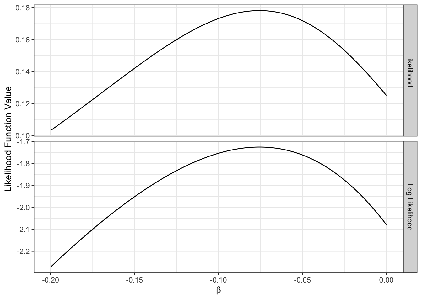

Figure 4.5: Likelihood and log-likelihood as a function of a parameter value.

---

1. These include numerical problems, because the MNP can only be calculated using multi-dimensional integration, and problems of interpretation. A special case of the MNP, when the error terms are distributed independently (no covariance) and identically (same variance), obtains estimation and prediction results that are very similar to those for the MNL model.↩︎

2. A model for which the probability can be calculated without use of numerical integration or simulation methods.↩︎

3. The exponent of a summation, \(\exp(A+B)\), is equal to the product of the exponents of the elements in the sum, \(\\exp(A) \exp(B)\) .↩︎

4. We use tables to illustrate calculation of the utility values and MNL probabilities. The first column shows the specification expression with appropriate values for variables and parameters, the second shows the calculated utility value, the third shows the exponent of the utility including the sum of the exponents, and the fourth shows the probability values.↩︎

5. This example ignores the increase in bus service frequency which might increase the probability of persons choosing bus; however, the increase is unlikely to be of the magnitude suggested by the IIA property.↩︎

6. In this case, we show the preservation of probabilities for the individual. In general, the individual probabilities are expected to change.↩︎

7. Interested readers are referred to train (1986) for a derivation and proof.↩︎

8. As before, interested readers are referred to Train (1986) for derivation and proof.↩︎

9. This comparison is independent of which alternative is chosen as the reference alternative since the effect of changing the reference alternative will be to increase each parameter by the same value.↩︎

10. Iso-utility lines connect all points for which the values of time and cost result in the same utility. The slope of these lines equals the inverse of the value of time, \(\beta_1/\beta_2\).↩︎

11. Dependence of \(P_{j't}\) on \(b\) is made implicit to simplify notation.↩︎

12. Dependence of \(P_{j't}\) on \(b\) is made implicit to simplify notation.↩︎