Chapter 3 Utility-based Choice Theory
3.1 Basic Construct of Utility Theory
Utility is an indicator of value to an individual. Generally, we think about utility as being derived from the attributes of alternatives or sets of alternatives; e.g., the total set of groceries purchased in a week. The utility maximization rule states that an individual will select the alternative from his/her set of available alternatives that maximizes his or her utility. Further, the rule implies that there is a function containing attributes of alternatives and characteristics of individuals that describes an individual’s utility valuation for each alternative. The utility function, \(U\), has the property that an alternative is chosen if its utility is greater than the utility of all other alternatives in the individual’s choice set. Alternatively, this can be stated as alternative, \('i'\), is chosen among a set of alternatives, if and only if the utility of alternative, \('i'\), is greater than or equal to the utility of all alternatives , \('j'\), in the choice set, \(C\). This can be expressed mathematically as:
\[\begin{equation} U(X_i,S_t) \geq U(X_j,S_t) \forall j \Rightarrow i \succ j \forall j \in C \tag{3.1} \end{equation}\]
where
- \(U(~~~)\) is the mathematical utility function,
- \(X_i,X_j\) are vectors of attributes describing alternatives i and j, respectively (e.g., travel time, travel cost, and other relevant attributes of the available modes),
- \(S_t\) is a vector of characteristics describing individual \(t\), that influence his/her preferences among alternatives (e.g., household income and number of automobiles owned for travel mode choice),
- \(i \succ j\) means the alternative to the left is preferred to the alternative to the right, and
- \(\forall j\) means all the cases, j, in the choice set.
That is, if the utility of alternative \(i\) is greater than or equal to the utility of all alternatives, \(j\); alternative \(i\) will be preferred and chosen from the set of alternatives, \(C\).
The underlying concept of utility allows us to rank a series of alternatives and identify the single alternative that has highest utility. The primary implication of this ranking or ordering of alternatives is that there is no absolute reference or zero point, for utility values. Thus, the only valuation that is important is the difference in utility between pairs of alternatives; particularly whether that difference is positive or negative. Any function that produces the same preference orderings can serve as a utility function and will give the same predictions of choice, regardless of the numerical values of the utilities assigned to individual alternatives. It also follows that utility functions, which result in the same order among alternatives, are equivalent.
3.2 Deterministic Choice Concepts
The utility maximization rule, which states that an individual chooses the alternative with the highest utility, implies no uncertainty in the individual’s decision process; that is, the individual is certain to choose the highest ranked alternative under the observed choice conditions. Utility models that yield certain predictions of choice are called deterministic utility models. The application of deterministic utility to the case of a decision between two alternatives is illustrated in Figure 3.1 that portrays a utility space in which the utilities of alternatives 1 and 2 are plotted along the horizontal and vertical axes, respectively, for each individual. The 45° line represents those points for which the utilities of the two alternatives are equal. Individuals B, C and D (above the equal-utility line) have higher utility for alternative 2 than for alternative 1 and are certain to choose alternative 2. Similarly, individuals A, E, and F (below the line) have higher utility for alternative 1 and are certain to choose that alternative. If deterministic utility models described behavior correctly, we would expect that an individual would make the same choice over time and that similar individuals (individuals having the same individual and household characteristics), would make the same choices when faced with the same set of alternatives. In practice, however, we observe variations in an individual’s choice and different choices among apparently similar individuals when faced with similar or even identical alternatives. For example, in studies of work trip mode choice, it is commonly observed that individuals, who are represented as having identical personal characteristics and who face the same sets of travel alternatives, choose different modes of travel to work. Further, some of these individuals vary their choices from day to day for no observable reason resulting in observed choices which appear to contradict the utility evaluations; that is, person A may choose Alternative 2 even though \(U_1 > U_2\) or person C may choose Alternative 2 even though \(U_2 > U_1\) . These observations raise questions about the appropriateness of deterministic utility models for modeling travel or other human behavior. The challenge is to develop a model structure that provides a reasonable representation of these unexplained variations in travel behavior.
tibble(U1 = c(2.5, 2, 3, 5, 6, 6),
       U2 = c(1, 4, 5, 7, 4, 5),
       label = c("A", "B", "C", "D", "E", "F")) %>%
  ggplot(aes(x = U1, y = U2, label = label)) +
  geom_point() +
  xlab("Utility for Alternative 1") +
  ylab("Utility for Alternative 2") +
  geom_abline(slope = 1, intercept = 0, lty = "dotted") +
  geom_label() +
  geom_text(data =
              tibble(U1 = c(2,5), U2 = c(6.5, 1.5),
                     label= c("Alt. 2 Preferred", "Alt. 1 Preferred"))) +
  scale_x_continuous(limits = c(0,8)) +
  scale_y_continuous(limits = c(0,8))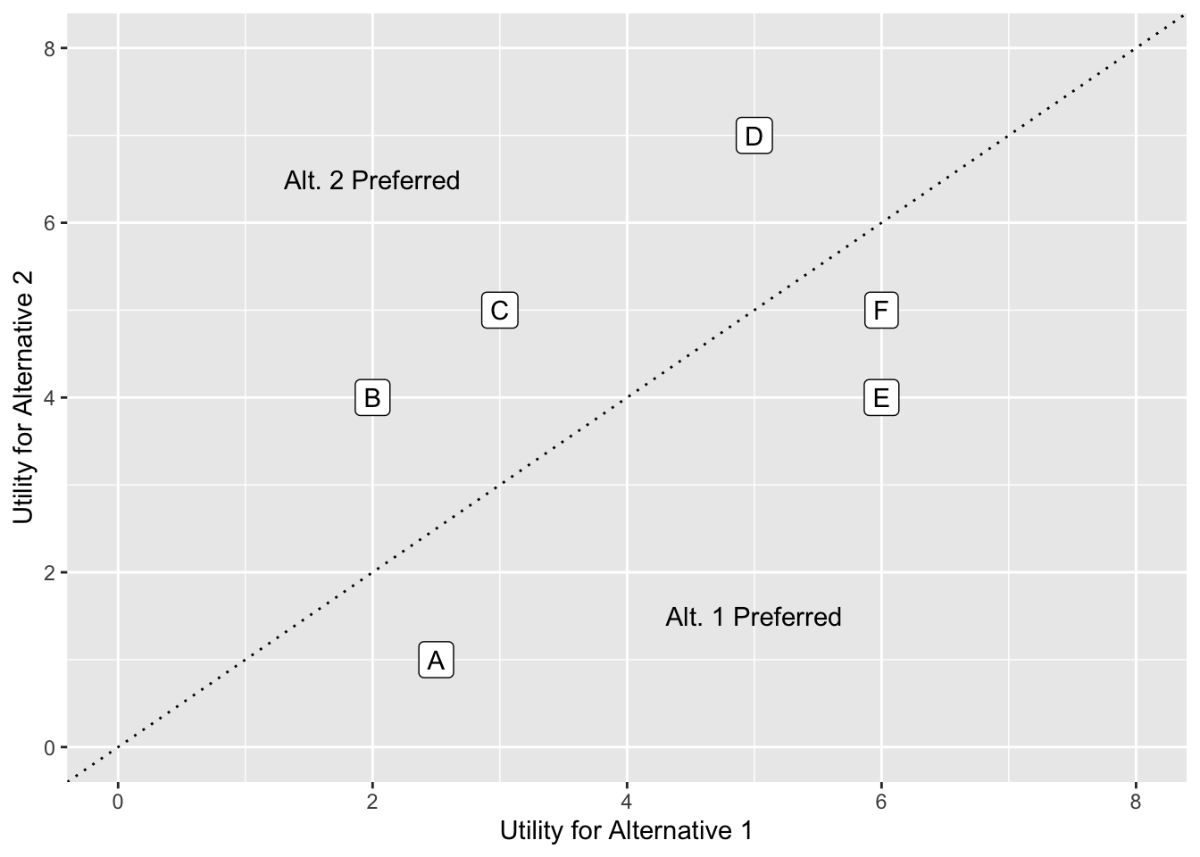
Figure 3.1: Illustration of Deterministic Choice
There are three primary sources of error in the use of deterministic utility functions. First, the individual may have incomplete or incorrect information or misperceptions about the attributes of some or all of the alternatives. As a result, different individuals, each with different information or perceptions about the same alternatives are likely to make different choices. Second, the analyst or observer has different or incomplete information about the same attributes relative to the individuals and an inadequate understanding of the function the individual uses to evaluate the utility of each alternative. For example, the analyst may not have good measures of the reliability of a particular transit service, the likelihood of getting a seat at a particular time of day or the likelihood of finding a parking space at a suburban rail station. However, the traveler, especially if he/she is a regular user, is likely to know these things or to have opinions about them. Third, the analyst is unlikely to know, or account for, specific circumstances of the individual’s travel decision. For example, an individual’s choice of mode for the work trip may depend on whether there are family visitors or that another family member has a special travel need on a particular day. Using models which do not account for and incorporate this lack of information results in the apparent behavioral inconsistencies described above. While human behavior may be argued to be inconsistent, it can also be argued that the inconsistency is only apparent and can be attributed to the analyst’s lack of knowledge regarding the individual’s decision making process. Models that take account of this lack of information on the part of the analyst are called random utility or probabilistic choice models.
3.3 Probabilistic Choice Theory
If analysts thoroughly understood all aspects of the internal decision making process of choosers as well as their perception of alternatives, they would be able to describe that process and predict mode choice using deterministic utility models. Experience has shown, however, that analysts do not have such knowledge; they do not fully understand the decision process of each individual or their perceptions of alternatives and they have no realistic possibility of obtaining this information. Therefore, mode choice models should take a form that recognizes and accommodates the analyst’s lack of information and understanding. The data and models used by analysts describe preferences and choice in terms of probabilities of choosing each alternative rather than predicting that an individual will choose a particular mode with certainty. Effectively, these probabilities reflect the population probabilities that people with the given set of characteristics and facing the same set of alternatives choose each of the alternatives.
As with deterministic choice theory, the individual is assumed to choose an alternative if its utility is greater than that of any other alternative. The probability prediction of the analyst results from differences between the estimated utility values and the utility values used by the traveler. We represent this difference by decomposing the utility of the alternative, from the perspective of the decision maker, into two components. One component of the utility function represents the portion of the utility observed by the analyst, often called the deterministic (or observable) portion of the utility. The other component is the difference between the unknown utility used by the individual and the utility estimated by the analyst. Since the utility used by the decision maker is unknown, we represent this difference as a random error. Formally, we represent this by:
\[\begin{equation} U_{it} = V_{it} + \epsilon_{it} \tag{3.2} \end{equation}\]
where
- \(U_{it}\) is the true utility of the alternative \(i\) to the decision maker \(t\), (\(U_{it}\)
is equivalent to \(U(X_i,S_t)\) but provides a simpler notation), - \(V_{it}\) is the deterministic or observable portion of the utility estimated by the analyst, and
- \(\epsilon_{it}\) is the error or the portion of the utility unkown to the analyst.
The analyst does not have any information about the error term. However, the total error which is the sum of errors from many sources (imperfect information, measurement errors, omission of modal attributes, omission of the characteristics of the individual that influence his/her choice decision and/or errors in the utility function) is represented by a random variable. Different assumptions about the distribution of the random variables associated with the utility of each alternative result in different representations of the model used to describe and predict choice probabilities. The assumptions used in the development of logit type models are discussed in the next Chapter.
3.4 Components of the Deterministic Portion of the Utility Function
The deterministic or observable portion (often called the systematic portion) of the utility of an alternative is a mathematical function of the attributes of the alternative and the characteristics of the decision maker. The systematic portion of utility can have any mathematical form but the function is most generally formulated as additive to simplify the estimation process. This function includes unknown parameters which are estimated in the modeling process. The systematic portion of the utility function can be broken into components that are (1) exclusively related to the attributes of alternatives, (2) exclusively related to the characteristics of the decision maker and (3) represent interactions between the attributes of alternatives and the characteristics of the decision maker. Thus, the systematic portion of utility can be represented by:
\[\begin{equation} V_{t,i} = V(S_t) + V(X_i) + V(S_t,X_i) \tag{3.3} \end{equation}\]
where
- \(V_{it}\) is the systematic portion of utility of alternative i for inidivual t,
- \(V(S_t)\) is the portion of utility associated with characteristics of individual
\(t\), - \(V(X_i)\) is the portion of utility of alternative \(i\) associated with the attributes of alternative \(i\), and
- \(V(S_t,X_i)\) is the portion of the utility which results from interactions between the attributes of alternative \(i\) and the characteristics of individual \(t\).
Each of these utility components is discussed separately
3.4.1 Utility Associated with the Attributes of Alternatives
The utility component associated exclusively with alternatives includes variables that describe the attributes of alternatives. These attributes influence the utility of each alternative for all people in the population of interest. The attributes considered for inclusion in this component are service attributes which are measurable and which are expected to influence people’s preferences/choices among alternatives. These include measures of travel time, travel cost, walk access distance, transfers required, crowding, seat availability, and others. For example: * Total travel time, * In-vehicle travel time, * Out-of-vehicle travel time, * Travel cost, * Number of transfers (transit modes), * Walk distance and, * Reliability of on time arrival. These measures differ across alternatives for the same individual and also among individuals due to differences in the origin and destination locations of each person’s travel. For example, this portion of the utility function could look like:
\[\begin{equation} V(X_i) = \gamma_1 ~ ' ~ X_{i1} + \gamma_2 ~ ' ~ X_{i2} + L + \gamma_k ~ ' ~ X_{ik} \tag{3.4} \end{equation}\]
where
- \(\gamma_k\) is the parameter which defines the direction and importance of the
effect of attribute \(k\) on the utility of an alternative and - \(X_{ik}\) is the value of attribute \(k\) for alternative \(i\).
Thus, this portion of the utility of each alternative, \(i\), is the weighted sum of the attributes of alternative \(i\). A specific example for the Drive Alone (DA), Shared Ride (SR), and Transit (TR) alternatives is:
\[\begin{equation} V(X_{DA}) = \gamma_1 ~ ' ~ TT_{DA} + \gamma_2 ~ ' ~ TC_{DA} \tag{3.5} \end{equation}\]
\[\begin{equation} V(X_{SR}) = \gamma_1 ~ ' ~ TT_{SR} + \gamma_2 ~ ' ~ TC_{SR} \tag{3.6} \end{equation}\]
\[\begin{equation} V(X_{TR}) = \gamma_1 ~ ' ~ TT_{TR} + \gamma_2 ~ ' ~ TC_{TR} + \gamma_3 ~ ' ~ FREQ_{TR} \tag{3.7} \end{equation}\]
where
- \(TT_i\) is the travel time for mode \(i\) (\(i\) = \(DA, SR, TR\)) and
- \(TC_i\) is the travel cost for mode \(i\), and
- \(FREQ_{TR}\) is the frequency for transit services.
Travel time and travel cost are generic; that is, they apply to all alternatives; frequency is specific to transit only. The parameters, \(\gamma_k\), are identical for all the alternatives to which they apply. This implies that the utility value of travel time and travel cost are identical across alternatives. The possibility that travel time may be more onerous on Transit than by Drive Alone or Shared Ride could be tested by reformulating the above models to:
\[\begin{equation} V(X_{DA}) = \gamma_{11} \times TT_{DA} + \gamma_{12} \times 0 + \gamma_2 \times TC_{DA} \tag{3.8} \end{equation}\]
\[\begin{equation} V(X_{SR}) = \gamma_{11} \times TT_{SR} + \gamma_{12} \times 0 + \gamma_2 \times TC_{SR} \tag{3.9} \end{equation}\]
\[\begin{equation} V(X_{TR}) = \gamma_{11} \times 0 + \gamma_{12} \times TT_{TR} + \gamma_2 \times TC_{TR} + \gamma_3 \times FREQ_{TR} \tag{3.10} \end{equation}\]
That is, two distinct parameters would be estimated for travel time; one for travel time by DA and SR, \(\gamma_{11}\), and the other for travel time by TR, \(\gamma_{12}\). These parameters could be compared to determine if the differences are statistically significant or large enough to be important.
3.4.2 Utility ‘Biases’ Due to Excluded Variables
It has been widely observed that decision makers exhibit preferences for alternatives which cannot be explained by the observed attributes of those alternatives. These preferences are described as alternative specific preference or bias; they measure the average preference of individuals with different characteristics for an alternative relative to a ‘reference’ alternative. As will be shown in CHAPTER 4, the selection of the reference alternative does not influence the interpretation of the model estimation results. In the simplest case, we assume that the bias is the same for all decision makers. In this case, this portion of the utility function would be:
\[\begin{equation} Bias_i = \beta_{i0} \times ASC_i \tag{3.11} \end{equation}\]
where \(\beta_{i0}\) represents an increase in the utility of alternative \(i\) for all choosers and \(ASC_i\) is equal to one for alternative \(i\) and zero for all other alternatives.
More detailed observation generally indicates that people with different personal and family characteristics have different preferences among sets of alternatives. For example, members of high income households are less likely to choose transit alternatives than low income individuals, all other things being equal. Similarly, members of households with fewer automobiles than workers are more likely to choose transit alternatives. Thus, it is useful to consider that the bias may differ across individuals as discussed in the next section.
3.4.4 Utility Defined by Interactions between Alternative Attributes and Decision Maker Characteristics
The final component of utility takes into account differences in how attributes are evaluated by different decision makers. One effect of income, described earlier, is to increase the preference for travel by private automobile. This representation implies that the preference for DA and SR increase with income, independent of the attributes of travel by each alternative. Another way to represent the influence of income is that increasing income reduces the importance of monetary cost in the evaluation of modal alternatives. The idea that high income travelers place less importance on cost can be represented by dividing the cost of travel of an alternative by annual income or some function of annual income of the traveler or his/her household. Another interaction effect might be that different travelers evaluate travel time differently. For example, one might argue that because women commonly take increased responsibility for home maintenance and child care, they are likely to evaluate increased travel time to work more negatively than men. This could be represented by adding a variable to the model which represents the product of a dummy variable for female (one if the traveler is a woman and zero otherwise) times travel time, as illustrated below in the utility equations for a three alternative mode choice example (Drive Alone, Shared Ride, and Transit) using the same notation described previously.
\[\begin{equation} V(X_{DA},S_{i})=\gamma_{1}\times TT_{DA}+\gamma_{2}\times TT_{DA}\times Fem+\gamma_{3}\times TC_{DA} \tag{3.16} \end{equation}\]
\[\begin{equation} V(X_{SR},S_{i})=\gamma_{1}\times TT_{SR}+\gamma_{2}\times TT_{SR}\times Fem+\gamma_{3}\times TC_{SR} \tag{3.17} \end{equation}\]
\[\begin{equation} V(X_{TR},S_{i})=\gamma_{1}\times TT_{TR}+\gamma_{2}\times TT_{TR}\times Fem+\gamma_{3}\times TC_{TR}+\gamma_{4}\times FREQ_{TR} \tag{3.18} \end{equation}\]
In this example, \(\gamma_1\) represents the utility value of one minute of travel time to men and \(\gamma_2\) represents the additional utility value of one minute of travel time to women. Thus, the total utility value of one minute of travel time to women is \(\gamma_1+\gamma_2\). In this case, \(\gamma_1\), is expected to be negative indicating that increased travel time reduces the utility of an alternative. \(\gamma_2\) may be negative or positive, indicating that women are more or less sensitive to increases in travel time.
3.5 Specification of the Additive Error Term
As described in section 3.3, the utility of each alternative is represented by a deterministic component, which is represented in the utility function by observed and measured variables, and an additive error term, \(\epsilon_i\) which represents those components of the utility function which are not included in the model. In the three alternative examples used above, the total utility of each alternative can be represented by:
\[\begin{equation} U_{DA}=V(S_t)+V(X_{DA})+V(S_t,X_{DA})+\epsilon_{DA} \tag{3.19} \end{equation}\]
\[\begin{equation} U_{SR}=V(S_t)+V(X_{SR})+V(S_t,X_{SR})+\epsilon_{SR} \tag{3.20} \end{equation}\]
\[\begin{equation} U_{TR}=V(S_t)+V(X_{TR})+V(S_t,X_{TR})+\epsilon_{TR} \tag{3.21} \end{equation}\]
where
- \(V()\) represents the deterministics components of the utility for the alternatives, and
- \(\epsilon_i\) represents the random components of the utility, also called the error term.
The error term is included in the utility function to account for the fact that the analyst is not able to completely and correctly measure or specify all attributes that determine travelers’ mode utility assessment. By definition, error terms are unobserved and unmeasured. A wide range of distributions could be used to represent the distribution of error terms over individuals and alternatives. If we assume that the error term for each alternative represents many missing components, each of which has relatively little impact on the value of each alternative, the central limit theorem suggests that the sum of these small errors will be distributed normally. This assumption leads to the formulation of the Multinomial Probit (MNP) probabilistic choice model. However, the mathematical complexity of the MNP model; which makes it difficult to estimate, interpret and predict; has limited its use in practice. An alternative distribution assumption, described in the next chapter, leads to the formulation of the multinomial logit (MNL) model.