Chapter 6 Model Specification Refinement: San Francisco Bay Area Work Mode Choice
# work trips data frame constructed in chapter 5
sf_mlogit <- read_rds("data/worktrips.rds")
6.1 Introduction
This chapter describes and demonstrates the refinement of the utility function specification for the multinomial logit (MNL) model for work mode choice in the San Francisco Bay Area. The process combines the use of intuition, statistical analysis and testing, and judgment. The intuition and judgment components of the model refinement process are based on theory, anecdotal evidence, logical analysis, and the accumulated empirical experience of the model developer. This empirical experience can be and often is enhanced through the advice of others or through review of reports and published papers documenting previous modeling studies for similar choice problems and contexts.
We explore a variety of different specifications of the utility functions to demonstrate some of the most common specifications and testing methods. These tests include both formal statistical tests and informal judgments about the signs, magnitudes, or relative magnitudes of parameters based on our knowledge about the underlying behavioral relationships that influence mode choice. The use of judgment and experience is an essential element of successful model development since it is almost impossible to determine the “best” model specification solely on the basis of statistical tests. A model that fits the data well may not necessarily describe the causal relationships and may not produce the most reasonable predictions. Also, it is not uncommon to find several model specifications that, for all practical purposes, fit the data equally well, but which have very different specifications and forecast implications. Therefore, practical model building involves considerable use of subjective judgment and is as much an art as it is a science.
Different modelers have different styles and approaches to the model development process. One of the most common approaches is to start with a minimal specification which includes those variables that are considered essential to any reasonable model. In the case of mode choice, such a specification might include travel time, travel cost and departure frequency where appropriate for each alternative. Working from this minimal specification, incremental changes are proposed and tested in an effort to improve the model in terms of its behavioral realism and/or its empirical fit to the data while avoiding excessive complexity of the model. Another common approach is to start with a richer specification which represents the model developer’s judgment about the set of variables that is likely to be included in the final model specification. For example, such a model might include travel time (separated into in-vehicle and out-of-vehicle time), out of vehicle travel time might be adjusted to take account of the total distance traveled, out of pocket travel cost (possibly adjusted by household income), frequency of departure for carrier modes, household automobile ownership or availability, household income, and size of the travel party.
We adopt the first of these methods in the following section for refinement of the specification of a model of work mode choice as it is the most appropriate approach for those who are new to discrete choice modeling. At each stage in the model development process, we introduce incremental changes to the modal utility functions and re-estimate the model with the objective of finding a more refined model specification that performs better statistically and is consistent with theory and our a priori expectations about mode choice behavior. We introduce small changes at each step as the estimation results for each stage provide useful insights which may be helpful in further refining the model. The appropriateness of each specification change is evaluated at each step using both judgmental and statistical tests. In the rest of this chapter, we describe and demonstrate this process for work mode choice in the San Francisco Bay Area.
6.2 Alternative Specifications
The basic multinomial logit mode choice model for work commute in the San Francisco Bay Area was reported in Table 5.4 in CHAPTER 5 . The refinements we consider include: - Different specifications of the income effects, - Different specifications of travel time, - Additional decision maker related variables such as gender and automobiles owned, - Additional variables that represent the interaction of decision maker related variables with mode related variables (e.g., interaction of income with cost), and - Additional trip context variables (e.g., dummy variable indicating if the trip origin/destination is in a Central Business District).
6.2.1 Refinement of Specification for Alternative Specific Income Effects
The estimation results for the base model in CHAPTER 5 yielded time and cost parameter estimates that had the expected (negative) sign and were statistically significant. The parameters for the alternative specific income variables were significant and had the expected sign (negative relative to drive alone) except for the shared ride specific income variables (shared ride 2 and shared ride 3+) which were not significant and the sign on the shared ride 3+ income variable was counter-intuitive. All else being equal, we expect the preference for shared ride 2 to be negative relative to drive alone and for shared ride 3+ to be more negative than shared ride 2 because of the increasing inconvenience of coordinating with other travelers as the number of persons in the ride sharing group increases. However, the empirical results provide only limited support for the first expectation and are inconsistent with the second expectation. This suggests that the effect of income on choice is not necessarily different among the automobile modes.
We approach this inconsistency between expectation and empirical results by thinking of other plausible relationships for the effect of income on shared ride choice and developing alternative specifications which represent these relationships. Options for consideration include:
- The effect of income relative to drive alone is the same for the two shared ride modes (shared ride 2 and shared ride 3+) but is different from drive alone and different from the other modes. This relationship is represented by constraining the income coefficients in the two shared alternatives to be equal as follows:
- The effect of income relative to drive alone is the same for both shared ride modes and transit but is different for the other modes. This is represented in the model by constraining the income coefficients in both shared ride modes and the transit mode to be equal as:
- The effect of income on all the automobile modes (drive alone, shared ride 2, and shared ride 3+) is the same, but the effect is different for the other modes. We include this constraint by setting the income coefficients in the utilities of the automobile modes to be equal. In this case, we set them to zero since drive alone is the reference mode.
\[\begin{equation} H_0 : \beta_{IncomeSR2} = \beta_{IncomeSR3+} = 0 \tag{6.3} \end{equation}\]
The estimation results for the base model (from CHAPTER 5) and for these three alternative models are reported in Table ??. The parameter estimates for all three models are consistent with expectations. That is, the effect of increasing income is neutral or negative for the shared ride modes relative to drive alone and equal to or more negative for transit, bike and walk than for shared ride. Further, all the parameters are significant except for the shared ride income parameters in Model 1W.
Selection of one of these four models to represent the effect of income should consider the statistical relationships among them and the reasonableness of the resultant models. Since Models 1W, 2W and 3W are constrained versions of the Base Model and Models 2W and 3W are constrained versions of Model 1W, we can use the likelihood ratio test to evaluate the hypotheses implied by each of these models (see section 5.7.3.2). We use this test to determine if the hypothesis that each of these models is the true model is or is not rejected by the less restricted model. The likelihood ratio statistics (Equation 5.16), the degrees of freedom or number of restrictions and the level of significance for each test are reported relative to the Base Model and to Model 1W in Table 6.2, respectively. The Base Model cannot reject any of the subsequent models at a reasonable level of significance. Further, the Base Model has a counter-intuitive relationship between the parameters for shared ride 2 and shared ride 3+. Thus, Model 1W or Model 3W can represent the effect of income on mode choice in this case. We choose Model 1W because it is most consistent with our prior hypotheses about the effect of income on preference between drive alone and shared ride and other modes. However, the differences among these models are small both statistically and behaviorally so the decision should be subject to a review before adoption of the final specification.27
model_base <- mlogit(chosen ~ tvtt + cost | hhinc, data = sf_mlogit, )
#Having issues setting Shared Ride 2 and 3+ to be equal to each other
model_1w <- mlogit(chosen ~ tvtt + cost | hhinc, data = sf_mlogit)
#Having issues setting Shared Ride 2, 3+, and Transit to be equal to each other
model_2w <- mlogit(chosen ~ tvtt + cost | hhinc, data = sf_mlogit)
model_3w <- mlogit(chosen ~ tvtt + cost | hhinc, data = sf_mlogit, constPar = c('hhinc:Share ride 2' = 0, 'hhinc:Share ride 3++' = 0))

altspecinc_estimation <- list(
  "Base Model " = model_base,
  "Model 1W" = model_1w,
  "Model 2W" = model_2w,
  "Model 3W" = model_3w
)

modelsummary(
  altspecinc_estimation, fmt = "%.4f",
  title = "Alternative Specifications of Income Variable"
)| Base Model | Model 1W | Model 2W | Model 3W | |
|---|---|---|---|---|
| (Intercept) × Share ride 2 | -2.1780 | -2.1780 | -2.1780 | -2.3043 |
| (0.1046) | (0.1046) | (0.1046) | (0.0547) | |
| (Intercept) × Share ride 3++ | -3.7251 | -3.7251 | -3.7251 | -3.7036 |
| (0.1777) | (0.1777) | (0.1777) | (0.0930) | |
| (Intercept) × Transit | -0.6709 | -0.6709 | -0.6709 | -0.6976 |
| (0.1326) | (0.1326) | (0.1326) | (0.1304) | |
| (Intercept) × Bike | -2.3763 | -2.3763 | -2.3763 | -2.3981 |
| (0.3045) | (0.3045) | (0.3045) | (0.3038) | |
| (Intercept) × Walk | -0.2068 | -0.2068 | -0.2068 | -0.2292 |
| (0.1941) | (0.1941) | (0.1941) | (0.1933) | |
| tvtt | -0.0513 | -0.0513 | -0.0513 | -0.0513 |
| (0.0031) | (0.0031) | (0.0031) | (0.0031) | |
| cost | -0.0049 | -0.0049 | -0.0049 | -0.0049 |
| (0.0002) | (0.0002) | (0.0002) | (0.0002) | |
| hhinc × Share ride 2 | -0.0022 | -0.0022 | -0.0022 | |
| (0.0016) | (0.0016) | (0.0016) | ||
| hhinc × Share ride 3++ | 0.0004 | 0.0004 | 0.0004 | |
| (0.0025) | (0.0025) | (0.0025) | ||
| hhinc × Transit | -0.0053 | -0.0053 | -0.0053 | -0.0049 |
| (0.0018) | (0.0018) | (0.0018) | (0.0018) | |
| hhinc × Bike | -0.0128 | -0.0128 | -0.0128 | -0.0125 |
| (0.0053) | (0.0053) | (0.0053) | (0.0053) | |
| hhinc × Walk | -0.0097 | -0.0097 | -0.0097 | -0.0093 |
| (0.0030) | (0.0030) | (0.0030) | (0.0030) | |
| Num.Obs. | 5029 | 5029 | 5029 | 5029 |
| AIC | 7276.4 | 7276.4 | 7276.4 | 7278.5 |
| BIC | ||||
| Log.Lik. | -3626.186 | -3626.186 | -3626.186 | -3627.234 |
| rho2 | 0.2534 | 0.2534 | 0.2534 | 0.2532 |
| rho20 | 0.5976 | 0.5976 | 0.5976 | 0.5975 |
| Model | loglik | lrtest | p_val |
|---|---|---|---|
| Model 1W | -3626.186 | 0.000000 | 1 |
| Model 2W | -3626.186 | 0.000000 | 1 |
| Model 3W | -3627.234 | 2.094772 | 0 |
6.2.2 Different Specifications of Travel Time
The specification for travel time in the above models implies that the utility value of time is equal for all the alternatives and between in-vehicle and out-of-vehicle time. However, we expect travelers in non-motorized modes to be more sensitive to travel time than travelers in motorized modes (since walking or biking is physically more demanding than traveling in a car) and we expect that travelers are more sensitive to out-of-vehicle travel time (OVT) than to in vehicle travel time (IVT).
The estimation results for two specifications of travel time that relax these constraints are reported with those for Model 1W in Table 6.3. Model 5W relaxes the time constraints in Model 1W by specifying distinct time variables for the motorized and non-motorized modes based on our expectation that travelers are likely to be more sensitive to travel time by non-motorized modes. Model 6W relaxes the constraint further by disaggregating the travel time for motorized modes into distinct components for IVT and OVT. This specification allows the two components of travel time for motorized travel to have different effects on utility with the expectation that travelers are more sensitive to out-of-vehicle time than in-vehicle time.
The estimation results for Model 5W rejects the hypothesis of equal value of travel time across modes implied in Model 1W and Model 6W rejects the hypothesis of equal value of in and out of travel time for the motorized modes at a very high level of significance \((0.001)\). The estimated parameters associated with travel time in Model 6W have the correct signs and the magnitude of the parameters for OVT for motorized modes and for time for non-motorized modes are larger in magnitude than the parameter for IVT, as expected; however, the parameter for IVT is very small and not statistically significant. Further, the ratio of OVT to IVT for motorized modes, 30 times, is far greater than expected. Nonetheless, since Model 6W rejects the constraints imposed by both Models 1W and 5W at a very high level of significance, we cannot discard this model without further exploration.
Another perspective on the suitability of these models can be obtained by calculating the relative importance of each component of travel time and cost which gives us the implied value of each component of time. The implied value of in-vehicle-time for motorized modes is computed for each model using the estimated motorized in-vehicle-time and cost parameters and similarly for the other time components:
\[\begin{equation} $\displaystyle = \text{Value of motorized IVTT (\$/hour)} = \frac{\beta_\text{motorized ivtt (1/min.)}}{\beta_{cost (1/cents)}} \times \frac{60 min./hour}{100 cents/\$} $ \tag{6.4} \end{equation}\]
The implied values of in- and out-of-vehicle times for motorized modes in Models 1W, 5W, and 6W are reported in Table 6.4. The values of motorized in-vehicle time and non-motorized time are somewhat low but not unreasonable compared to the average wage rate of $21.20 per hour in the region (1990 dollars); however, the value of in-vehicle time is unreasonably low. Nevertheless, the likelihood ratio tests reject both Model 5W and Model 1W at very high levels of significance. This raises doubt about the suitability of those models and suggests the need to consider other specifications to evaluate the influence of travel time components on the utilities of the different alternatives.
Two approaches are commonly taken to identify a specification which is not statistically rejected by other models and has good behavioral relationships among variables. The first is to examine a range of different specifications in an attempt to find one which is both behaviorally sound and statistically supported. The other is to constrain the relationships between or among parameter values to ratios which we are considered reasonable. The formulation of these constraints is based on the judgment and prior empirical experience of the analyst. Therefore, the use of such constraints imposes a responsibility on the analyst to provide a sound basis for his/her decision. The advice of other more experienced analysts is often enlisted to expand and/or support these judgments.
#Having issues setting Shared Ride 2 and 3+ to be equal to each other
model_5w <- mlogit(chosen ~ mot_tvtt + nm_tvtt + cost | hhinc, data = sf_mlogit)
#Having issues setting Shared Ride 2 and 3+ to be equal to each other
model_6w <- mlogit(chosen ~ nm_tvtt + mot_ovtt + mot_ivtt + cost | hhinc, data = sf_mlogit)

altspectvtt_estimation <- list(
  "Model 1W" = model_1w,
  "Model 5W" = model_5w,
  "Model 6W" = model_6w
)

modelsummary(
  altspectvtt_estimation, fmt = "%.4f",
  title = "Estimation Results for Alternative Specifications of Travel Time[^trumodel], [^valuesoftime]"
)| Model 1W | Model 5W | Model 6W | |
|---|---|---|---|
| (Intercept) × Share ride 2 | -2.1780 | -2.2279 | -2.3961 |
| (0.1046) | (0.1052) | (0.1075) | |
| (Intercept) × Share ride 3++ | -3.7251 | -3.7897 | -3.9957 |
| (0.1777) | (0.1782) | (0.1802) | |
| (Intercept) × Transit | -0.6709 | -0.8532 | -0.4910 |
| (0.1326) | (0.1392) | (0.1490) | |
| (Intercept) × Bike | -2.3763 | -1.8437 | -1.7186 |
| (0.3045) | (0.3258) | (0.3231) | |
| (Intercept) × Walk | -0.2068 | 0.4773 | 0.4096 |
| (0.1941) | (0.2522) | (0.2533) | |
| tvtt | -0.0513 | ||
| (0.0031) | |||
| cost | -0.0049 | -0.0050 | -0.0048 |
| (0.0002) | (0.0002) | (0.0002) | |
| hhinc × Share ride 2 | -0.0022 | -0.0021 | -0.0022 |
| (0.0016) | (0.0016) | (0.0016) | |
| hhinc × Share ride 3++ | 0.0004 | 0.0004 | 0.0003 |
| (0.0025) | (0.0025) | (0.0025) | |
| hhinc × Transit | -0.0053 | -0.0054 | -0.0057 |
| (0.0018) | (0.0018) | (0.0019) | |
| hhinc × Bike | -0.0128 | -0.0125 | -0.0122 |
| (0.0053) | (0.0053) | (0.0052) | |
| hhinc × Walk | -0.0097 | -0.0095 | -0.0093 |
| (0.0030) | (0.0031) | (0.0031) | |
| mot_tvtt | -0.0431 | ||
| (0.0035) | |||
| nm_tvtt | -0.0687 | -0.0632 | |
| (0.0053) | (0.0054) | ||
| mot_ovtt | -0.0759 | ||
| (0.0059) | |||
| mot_ivtt | -0.0025 | ||
| (0.0062) | |||
| Num.Obs. | 5029 | 5029 | 5029 |
| AIC | 7276.4 | 7259.0 | 7203.3 |
| BIC | |||
| Log.Lik. | -3626.186 | -3616.494 | -3587.643 |
| rho2 | 0.2534 | 0.2554 | 0.2614 |
| rho20 | 0.5976 | 0.5986 | 0.6018 |
| Value of Time ($/hr) | Model 1W | Model 5W | Model 6W |
|---|---|---|---|
| Value of Non-Motorized Time | 6.26 | 8.24 | 7.91 |
| Value of Out-of-vehicle Time | 6.26 | 5.17 | 9.50 |
| Value of In-vehicle Time | 6.26 | 5.17 | 0.32 |
The primary shortcoming of the specification in Model 6W is that the estimated value of IVT is unrealistically small. At least two alternatives can be considered for getting an improved estimate of the value of out-of-vehicle time. One is to use an approach that has been effective in other contexts; that is, to assume that the sensitivity of travelers to OVT diminishes with the trip distance. The idea behind this is that travelers are more willing to tolerate higher out-of-vehicle time for a long trip rather than for a short trip. We still expect that travelers will be more sensitive to OVT than IVT for any travel distance. A formulation which ensures this result is to include total travel time (the sum of in-vehicle and out-of-vehicle time) and out-of-vehicle time divided by distance in place of in- and out-of-vehicle travel time. This specification, as shown below, is consistent with our expectations provided that \(\beta_1\) and \(\beta_2\) are negative:
\[\begin{equation} \begin{split} V_{m} &= \gamma_{0,m} + \beta_{1} \times TTT_{m} + \beta_{2} \times \Big(\frac{OVT_{m}}{Dist}\Big) + \ldots\\ &= \gamma_{0,m} + \beta_{1} \times (IVT_{m} + OVT_{m}) + \frac{\beta_{2}}{Dist} \times OVT_{m} + \ldots\\ &= \gamma_{0,m} + \beta_{1} \times IVT_{m} + \Big(\beta_{1} + \frac{\beta_{2}}{Dist}\Big) \times OVT_{m} + \ldots \end{split} \tag{6.5} \end{equation}\]
An alternative approach is to impose a constraint on the relative importance of OVT and IVT. This is achieved by replacing the travel time variables in the modal utility equations with a weighted travel time (WTT) variable defined as in-vehicle time plus the appropriate travel time importance ratio (TIR) times out-of-vehicle time (IVT + TIR×OVT). The mechanics of how this constraint works is illustrated as follows:
\[\begin{equation} \begin{split} V_{m} &= \gamma_{0,m} + \beta_{1} \times IVT + (\beta_{1} \times TIR) \times OVT + \ldots \\ &= \gamma_{0,m} + \beta_{1} \times (IVT + TIR \times OVT) + \ldots\\ &= \gamma_{0,m} + \beta_{1} \times WTT + \ldots \end{split} \tag{6.6} \end{equation}\]
so that the parameter for out-of-vehicle time is equal to the parameter for in-vehicle time multiplied by the selected travel time ratio (TTR). In Models 8W and 9W, we use travel importance ratios of 2.5 and 4.0, respectively. The estimation results for these models compared to Model 6W are reported in Table 6-5. The parameter estimates obtained for the travel time, cost, and income variables in all four models have the correct signs and are statistically significant. Model 7W has substantially better goodness-of-fit than Models 6W, 8W and 9W. Since none of the other models are constrained versions of Model 7W, we use the non-nested hypothesis test (see Section 5.7.3.2, Equation 5.21) to compare it with Models 6W, 8W, and 9W.
We illustrate the non-nested hypothesis test by applying it to the hypothesis that Model 6W is the true model given that Model 7W has a higher \(\bar{\rho}^{2}\). Since both models have the same number of parameters, the term (K7-K6) drops out, and the equation becomes
\[\begin{equation} \begin{split} \mathrm{Level of Rejection} &= \Phi[-(-2(\bar{\rho_{7}}^{2}-\bar{\rho_{6}}^{2})\ l(0))^{1/2}]\\ &= \Phi[-(-2(0.5129-0.5074)(-7309.6))^{1/2}]\\ &= \Phi(-8.97)<< 0.001 \end{split} \tag{6.7} \end{equation}\]
That is, the null hypothesis that Model 6W is the true model is rejected with significance much greater than \(0.001\). Models 8W and 9W are also rejected as the true model at an even higher level of significance.
sf_mlogit_trip_estimates <- sf_mlogit %>%
  mutate(
    TIR8 = (mot_ivtt + 2.4 * mot_ovtt),
    TIR9 = (mot_ivtt + 4 * mot_ovtt),
    ovtd = mot_ovtt/dist,
    scalemot = 2.4 * mot_ovtt,
    scalemot2 = 4 * mot_ovtt
    )

model_7w <- mlogit(chosen ~ mot_tvtt + nm_tvtt + ovtd + cost | hhinc,
                   data = sf_mlogit_trip_estimates)
model_8w <- mlogit(chosen ~ nm_tvtt + TIR8  + cost | hhinc,
                   data = sf_mlogit_trip_estimates)
model_9w <- mlogit(chosen ~ nm_tvtt + TIR9 + cost | hhinc,
                   data = sf_mlogit_trip_estimates)
model_8a <- mlogit(chosen ~ nm_tvtt + (mot_ivtt + scalemot) + cost | hhinc,
                    data = sf_mlogit_trip_estimates)
model_9a <- mlogit(chosen ~ nm_tvtt + (mot_ivtt + scalemot2) + cost | hhinc,
data = sf_mlogit_trip_estimates)| Model 6W | Model 7W | Model 8W | Model 9W | |
|---|---|---|---|---|
| (Intercept) × Share ride 2 | -2.3961 | -2.1519 | -2.2923 | -2.3302 |
| (0.1075) | (0.1047) | (0.1042) | (0.1039) | |
| (Intercept) × Share ride 3++ | -3.9957 | -3.6362 | -3.8650 | -3.9120 |
| (0.1802) | (0.1758) | (0.1772) | (0.1768) | |
| (Intercept) × Transit | -0.4910 | -0.0431 | -0.5897 | -0.5281 |
| (0.1490) | (0.1597) | (0.1462) | (0.1479) | |
| (Intercept) × Bike | -1.7186 | -2.6862 | -1.8035 | -1.7741 |
| (0.3231) | (0.3337) | (0.3240) | (0.3232) | |
| (Intercept) × Walk | 0.4096 | -1.0226 | 0.4439 | 0.4297 |
| (0.2533) | (0.2920) | (0.2524) | (0.2526) | |
| nm_tvtt | -0.0632 | -0.0475 | -0.0664 | -0.0652 |
| (0.0054) | (0.0055) | (0.0053) | (0.0053) | |
| mot_ovtt | -0.0759 | |||
| (0.0059) | ||||
| mot_ivtt | -0.0025 | |||
| (0.0062) | ||||
| cost | -0.0048 | -0.0041 | -0.0049 | -0.0048 |
| (0.0002) | (0.0002) | (0.0002) | (0.0002) | |
| hhinc × Share ride 2 | -0.0022 | -0.0020 | -0.0022 | -0.0022 |
| (0.0016) | (0.0015) | (0.0016) | (0.0016) | |
| hhinc × Share ride 3++ | 0.0003 | 0.0006 | 0.0004 | 0.0003 |
| (0.0025) | (0.0025) | (0.0025) | (0.0025) | |
| hhinc × Transit | -0.0057 | -0.0072 | -0.0055 | -0.0055 |
| (0.0019) | (0.0019) | (0.0018) | (0.0018) | |
| hhinc × Bike | -0.0122 | -0.0119 | -0.0124 | -0.0123 |
| (0.0052) | (0.0052) | (0.0053) | (0.0052) | |
| hhinc × Walk | -0.0093 | -0.0082 | -0.0095 | -0.0094 |
| (0.0031) | (0.0032) | (0.0031) | (0.0031) | |
| mot_tvtt | -0.0415 | |||
| (0.0035) | ||||
| ovtd | -0.1813 | |||
| (0.0179) | ||||
| TIR8 | -0.0262 | |||
| (0.0019) | ||||
| TIR9 | -0.0173 | |||
| (0.0013) | ||||
| Num.Obs. | 5029 | 5029 | 5029 | 5029 |
| AIC | 7203.3 | 7121.8 | 7216.8 | 7207.0 |
| BIC | ||||
| Log.Lik. | -3587.643 | -3546.891 | -3595.381 | -3590.518 |
| rho2 | 0.2614 | 0.2698 | 0.2598 | 0.2608 |
| rho20 | 0.6018 | 0.6064 | 0.6010 | 0.6015 |
Before adopting Model 7W, it is a good idea to evaluate and interpret the relative importance of in-vehicle and out-of-vehicle time and between each component of time and cost. Despite the difference in the specification, this analysis is undertaken the same way as earlier; that is, the parameters for time is divided by the parameter for cost to obtain the values of time. The values of IVT and OVT in cents-per-minute (and dollars-per-hour) are shown in Table 6.6 as a function of distance. The time values are obtained as described earlier by dividing each of the time parameters (in utils-per-minute) by the cost parameter in utils per cent. For example, the values for Model 7W are:
Value of IVTT \(= \frac{\beta_{mot\ tvtt}}{\beta_{cost}} = \frac{-0.0415}{-0.0041}\) = 10.1 cents/min = $6.07/hr
Value of OVT (5 Mile Trip) \(= \frac{\beta_{mot\ tvtt}+ \frac{\beta_{OVT/Dist}}{Dist}}{\beta_{cost}}\) \(= \frac{-0.0415+ \frac{-0.1812}{5}}{-0.0041}\) = 19.0 cents/min = $11.38/hr
These values of time are fixed for IVT but vary with distance for OVT30 as reported in Table 6.6 for Model 7W. The corresponding values of time for Models 6W, 8W and 9W are shown in Table ??
| distance | Value of Motorized Out-of-Vehicle Time | Value of Motorized Total Time | Value of Non-Motorized Time |
|---|---|---|---|
| 5 | NA | 10.10156 | 11.53997 |
| 10 | NA | 10.10156 | 11.53997 |
| 20 | NA | 10.10156 | 11.53997 |
| Value of Time ($/hr) | Model 6W | Model 8W | Model 9W |
|---|---|---|---|
| Value of Out-of-vehicle Time | 9.50 | NA | NA |
| Value of In-vehicle Time | 0.32 | NA | NA |
The prevailing wage rate in the San Francisco Bay Area is $21.20 per hour31. In comparison, the values of in-vehicle time implied by Models 6W, 8W, and 9W are very low and the values of out of vehicle time are somewhat low. Model 7W produces higher, but still low, values of time. Finally, we can examine the ratio of time values of OVT relative to IVT for all four models as shown in Figure 6.1. The ratio for Model 6W is unacceptably high. Those for Models 7W, 8W and 9W are more reasonable.
vottable <- tibble(
  model = c("Model 6W", "Model 7W", "Model 8W", "Model 9W"),
  ovtt = c( VOTsimple(model_6w, "mot_ovtt", "cost"), VOTsimple(model_7w, "mot_tvtt", "cost"),
            VOTsimple(model_8a, "scalemot", "cost"), VOTsimple(model_9a, "scalemot2", "cost")),
  ivtt =  c(VOTsimple(model_6w, "mot_ivtt", "cost"), VOTsimple(model_7w, "mot_tvtt", "cost"),
            VOTsimple(model_8a, "mot_ivtt", "cost"), VOTsimple(model_9a, "mot_ivtt", "cost")),
  ratio = ovtt / ivtt
)

tibble(
  distance = .8:10,
  `Model 6W` = vottable$ratio[1],
  `Model 7W` = vottable$ratio[2] / distance,
  `Model 8W` = vottable$ratio[3],
  `Model 9W` = vottable$ratio[4],
) %>%
  gather(model, vot, -distance) %>%
  ggplot(aes(x = distance, y = vot, color = model)) +
  scale_color_discrete("Model") +
  geom_line()  + xlab("Distance") + ylab("Value of Time Ratio") +
  scale_y_log10()
## Warning: attributes are not identical across measure variables;
## they will be dropped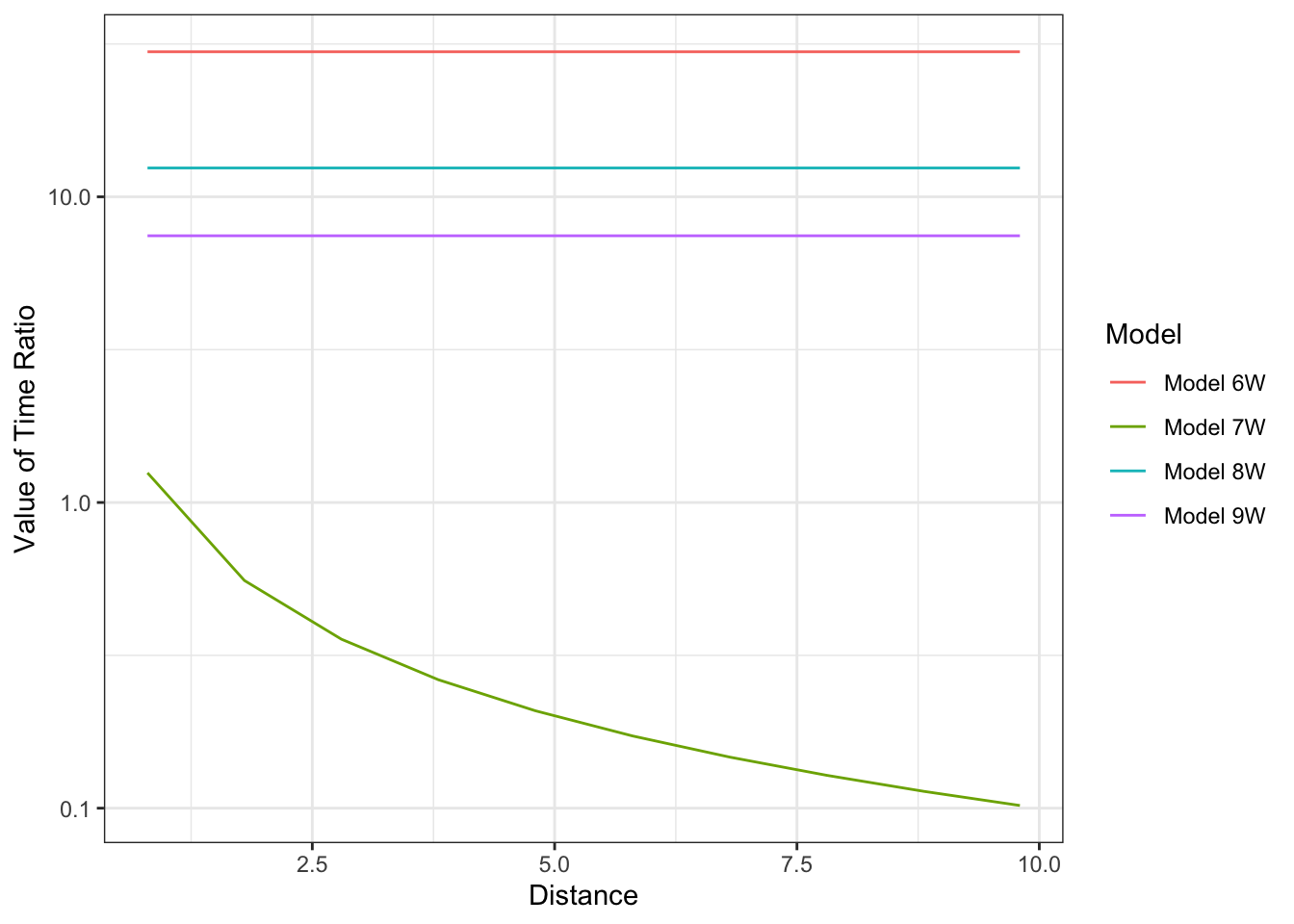
Figure 6.1: Ratio of Out-of-Vehicle and In-Vehicle Time Coefficients for Work Models 6, 7, 8, and 9
The selection of a preferred travel time specification among the four alternative specifications tested is relatively straightforward in this case. Model 7W outperforms the other models in all the evaluations undertaken; it has the best goodness-of-fit, the most intuitive relationship between the IVT and OVT variables and the most acceptable values of time32. Consequently, Model 7W is our preferred travel time specification. We can still consider imposing a constraint between the time and cost variables to force the value of time to more reasonable levels. However, we defer this until we explore other specification improvements.
6.2.4 Including Trip Context variables
The models considered to this point include variables that describe the attributes of alternatives, modes, and the characteristics of decision-makers (the work commuters). The mode choice decision also is influenced by variables that describe the context in which the trip is made. For example, a work trip to the regional central business district (CBD) is more likely to be made by transit than an otherwise similar trip to a suburban work place because the CBD is generally well-served by transit, has more opportunities to make additional stops by walking and is less auto friendly due to congestion and limited and expensive parking. This suggests that the model specification can be enhanced by including variables related to the context of the trip, such as destination zone location.
We consider two distinct variables to describe the trip destination context. One is a dummy variable which indicates whether the destination zone (workplace) is located in the CBD; the other is the employment density of different workplace destinations. The CBD variable implies an abrupt increase in the likelihood of using public transit at the CBD boundary. The density variable implies a continuous increase in the likelihood of using public transit with increasing workplace density. A third option is to include both variables in the model. There is disagreement about whether to include such combinations of variables since they both represent the same underlying phenomenon: increasing transit use with increasing density of development. There is no firm rule about this point; each case must be evaluated on its merits based on statistical tests and reasonableness of the estimation results. As with the addition of characteristics of the traveler, we introduce each variable as a full set of alternative specific variables, each of which represents the effect of a change in that variable on the utility of the alternative relative to the reference alternative (drive alone). Model 13W adds the alternative specific CBD dummy variables to the variables in Model 11W. Model 14W adds the alternative specific employment density variables and Model 15W adds both. Estimation results for these specifications and Model 11W are reported in Table 6-9.
## Warning in sanity_ellipsis(vcov, ...): The `statistic_vertical` argument
## is deprecated and will be ignored. To display uncertainty estimates next to
## your coefficients, use a `glue` string in the `estimate` argument. See `?
## modelsummary`| Model 11W | Model 13W | Model 14W | Model 15W | |
|---|---|---|---|---|
| (Intercept) × Share ride 2 | -1.5651 | -1.6134 | -1.5818 | -1.6192 |
| (0.1364) | (0.1403) | (0.1370) | (0.1403) | |
| (Intercept) × Share ride 3++ | -3.2375 | -3.6071 | -3.2913 | -3.6182 |
| (0.2195) | (0.2333) | (0.2219) | (0.2333) | |
| (Intercept) × Transit | 0.9262 | -0.2034 | 0.4180 | -0.4729 |
| (0.1924) | (0.2426) | (0.2090) | (0.2512) | |
| (Intercept) × Bike | -1.8303 | -1.6502 | -1.5966 | -1.5145 |
| (0.4082) | (0.4284) | (0.4170) | (0.4296) | |
| (Intercept) × Walk | -0.2371 | 0.0845 | -0.0399 | 0.2108 |
| (0.3410) | (0.3476) | (0.3442) | (0.3483) | |
| mot_tvtt | -0.0384 | -0.0286 | -0.0299 | -0.0231 |
| (0.0036) | (0.0038) | (0.0038) | (0.0039) | |
| nm_tvtt | -0.0470 | -0.0464 | -0.0459 | -0.0467 |
| (0.0056) | (0.0057) | (0.0057) | (0.0058) | |
| mot_ovttbydist | -0.1814 | -0.1501 | -0.1575 | -0.1324 |
| (0.0185) | (0.0197) | (0.0190) | (0.0197) | |
| cost | -0.0042 | -0.0033 | -0.0029 | -0.0024 |
| (0.0002) | (0.0003) | (0.0003) | (0.0003) | |
| hhinc × Share ride 2 | -0.0022 | -0.0022 | -0.0022 | -0.0022 |
| (0.0016) | (0.0016) | (0.0016) | (0.0016) | |
| hhinc × Share ride 3++ | 0.0001 | -0.0004 | -0.0003 | -0.0005 |
| (0.0025) | (0.0025) | (0.0025) | (0.0025) | |
| hhinc × Transit | -0.0060 | -0.0061 | -0.0070 | -0.0070 |
| (0.0020) | (0.0020) | (0.0020) | (0.0021) | |
| hhinc × Bike | -0.0116 | -0.0111 | -0.0112 | -0.0109 |
| (0.0053) | (0.0052) | (0.0053) | (0.0053) | |
| hhinc × Walk | -0.0080 | -0.0078 | -0.0079 | -0.0081 |
| (0.0032) | (0.0032) | (0.0032) | (0.0032) | |
| vehbywrk × Share ride 2 | -0.4298 | -0.4129 | -0.4044 | -0.3988 |
| (0.0767) | (0.0769) | (0.0764) | (0.0769) | |
| vehbywrk × Share ride 3++ | -0.2732 | -0.2175 | -0.2423 | -0.1880 |
| (0.1129) | (0.1114) | (0.1133) | (0.1111) | |
| vehbywrk × Transit | -0.9903 | -0.9113 | -0.9956 | -0.9303 |
| (0.1157) | (0.1148) | (0.1190) | (0.1179) | |
| vehbywrk × Bike | -0.6731 | -0.6982 | -0.7137 | -0.7151 |
| (0.2515) | (0.2561) | (0.2585) | (0.2590) | |
| vehbywrk × Walk | -0.6286 | -0.7197 | -0.6815 | -0.7276 |
| (0.1627) | (0.1682) | (0.1671) | (0.1694) | |
| cbddumall × Share ride 2 | 0.2571 | 0.2037 | ||
| (0.1100) | (0.1246) | |||
| cbddumall × Share ride 3++ | 1.0520 | 1.0161 | ||
| (0.1725) | (0.1926) | |||
| cbddumall × Transit | 1.3556 | 1.2037 | ||
| (0.1613) | (0.1678) | |||
| cbddumall × Bike | 0.3755 | 0.4609 | ||
| (0.3214) | (0.3601) | |||
| cbddumall × Walk | 0.1740 | 0.1074 | ||
| (0.2252) | (0.2508) | |||
| wkempden × Share ride 2 | 0.0011 | 0.0010 | ||
| (0.0004) | (0.0004) | |||
| wkempden × Share ride 3++ | 0.0022 | 0.0013 | ||
| (0.0004) | (0.0005) | |||
| wkempden × Transit | 0.0027 | 0.0021 | ||
| (0.0004) | (0.0004) | |||
| wkempden × Bike | 0.0011 | 0.0008 | ||
| (0.0011) | (0.0012) | |||
| wkempden × Walk | 0.0015 | 0.0018 | ||
| (0.0007) | (0.0008) | |||
| Num.Obs. | 5029 | 5029 | 5029 | 5029 |
| AIC | 7015.8 | 6928.9 | 6968.9 | 6906.7 |
| BIC | ||||
| Log.Lik. | -3488.886 | -3440.445 | -3460.438 | -3424.361 |
| rho2 | 0.2817 | 0.2917 | 0.2876 | 0.2950 |
| rho20 | 0.6128 | 0.6182 | 0.6160 | 0.6200 |
| Value of Time ($/hr) | Model 13W | Model 14W | Model 15W |
|---|---|---|---|
| Value of Motorized IVT | 5.23 | 6.22 | 5.88 |
| Value of Motorized OVT (10 mile trip) | 7.97 | 9.50 | 9.25 |
| Value of Motorized OVT (20 mile trip) | 6.60 | 7.86 | 7.57 |
| Value of Non-Motorized Time | 8.48 | 9.54 | 11.89 |
Each of the new Models (13W, 14W and 15W) significantly reject Model 11W as the true model at a very high level of significance. Further, the parameters for all of the alternative specific CBD dummy and employment density variables have a positive sign, implying that all else being equal, an individual is less likely to choose drive alone mode for trips destined to a CBD and/or high employment density zones, as expected.
Since Models 13W and 14W are restricted versions of Model 15W, we can use the loglikelihood test which rejects the hypothesis that each of these models is the true model. Therefore, purely on statistical grounds, Model 15W is preferred over Models 13W and 14W. However, this improvement in statistical fit comes at the cost of increased model complexity, and it may be appropriate to adopt Model 13W or 14W, sacrificing statistical fit in favor of parsimony33. For now, we choose Model 15W as the preferred model for its stronger statistical results, but we will return to the issue of model complexity.
6.2.5 Interactions between Trip maker and/or Context Characteristics and Mode Attributes
Another approach to the inclusion of trip maker or context characteristics is through interactions with mode attributes. The most common example of this approach is to take account of the expectation that low-income travelers will be more sensitive to travel cost than high-income travelers by using cost divided by income in place of cost as an explanatory variable. Such a specification implies that the importance of cost in mode choice diminishes with increasing household income. Table 6-11 portrays the estimation results for two models that differ only in how they represent cost; Model 15W includes travel cost while Model 16W includes travel cost divided by income.
## Warning in sanity_ellipsis(vcov, ...): The `statistic_vertical` argument
## is deprecated and will be ignored. To display uncertainty estimates next to
## your coefficients, use a `glue` string in the `estimate` argument. See `?
## modelsummary`| Model 15W | Model 16W | |
|---|---|---|
| (Intercept) × Share ride 2 | -1.6192 | -1.6976 |
| (0.1403) | (0.1419) | |
| (Intercept) × Share ride 3++ | -3.6182 | -3.7733 |
| (0.2333) | (0.2356) | |
| (Intercept) × Transit | -0.4729 | -0.6930 |
| (0.2512) | (0.2496) | |
| (Intercept) × Bike | -1.5145 | -1.6233 |
| (0.4296) | (0.4290) | |
| (Intercept) × Walk | 0.2108 | 0.0751 |
| (0.3483) | (0.3492) | |
| mot_tvtt | -0.0231 | -0.0202 |
| (0.0039) | (0.0038) | |
| nm_tvtt | -0.0467 | -0.0455 |
| (0.0058) | (0.0058) | |
| mot_ovttbydist | -0.1324 | -0.1326 |
| (0.0197) | (0.0196) | |
| cost | -0.0024 | |
| (0.0003) | ||
| hhinc × Share ride 2 | -0.0022 | -0.0006 |
| (0.0016) | (0.0016) | |
| hhinc × Share ride 3++ | -0.0005 | 0.0023 |
| (0.0025) | (0.0025) | |
| hhinc × Transit | -0.0070 | -0.0052 |
| (0.0021) | (0.0021) | |
| hhinc × Bike | -0.0109 | -0.0086 |
| (0.0053) | (0.0052) | |
| hhinc × Walk | -0.0081 | -0.0060 |
| (0.0032) | (0.0032) | |
| vehbywrk × Share ride 2 | -0.3988 | -0.3780 |
| (0.0769) | (0.0765) | |
| vehbywrk × Share ride 3++ | -0.1880 | -0.1475 |
| (0.1111) | (0.1101) | |
| vehbywrk × Transit | -0.9303 | -0.9400 |
| (0.1179) | (0.1185) | |
| vehbywrk × Bike | -0.7151 | -0.7046 |
| (0.2590) | (0.2586) | |
| vehbywrk × Walk | -0.7276 | -0.7240 |
| (0.1694) | (0.1696) | |
| cbddumall × Share ride 2 | 0.2037 | 0.2458 |
| (0.1246) | (0.1241) | |
| cbddumall × Share ride 3++ | 1.0161 | 1.0923 |
| (0.1926) | (0.1909) | |
| cbddumall × Transit | 1.2037 | 1.3024 |
| (0.1678) | (0.1657) | |
| cbddumall × Bike | 0.4609 | 0.4829 |
| (0.3601) | (0.3613) | |
| cbddumall × Walk | 0.1074 | 0.0936 |
| (0.2508) | (0.2524) | |
| wkempden × Share ride 2 | 0.0010 | 0.0016 |
| (0.0004) | (0.0004) | |
| wkempden × Share ride 3++ | 0.0013 | 0.0022 |
| (0.0005) | (0.0005) | |
| wkempden × Transit | 0.0021 | 0.0031 |
| (0.0004) | (0.0004) | |
| wkempden × Bike | 0.0008 | 0.0019 |
| (0.0012) | (0.0012) | |
| wkempden × Walk | 0.0018 | 0.0029 |
| (0.0008) | (0.0007) | |
| I(cost/hhinc) | -0.0528 | |
| (0.0108) | ||
| Num.Obs. | 5029 | 5029 |
| AIC | 6906.7 | 6941.6 |
| BIC | ||
| Log.Lik. | -3424.361 | -3441.782 |
| rho2 | 0.2950 | 0.2914 |
| rho20 | 0.6200 | 0.6180 |
The cost by income variable has the expected sign and is statistically significant, but the overall goodness-of-fit for the cost divided by income model is lower than that for model 15 that uses cost without interaction with income. However, because theory and common sense suggest that the importance of cost should decrease with income, we may choose Model 16W despite the differences in the goodness-of-fit statistics. Since the estimation results contradict our understanding of the decision making behavior, it is useful to consider other aspects of model results. In the case of mode choice, we are particularly interested in the relative value of the time and cost parameters because it measures the implied value of time used by travelers in choosing their travel mode. Values of time evaluated with earlier models were somewhat lower than expected when compared to the average wage rate. Using the cost by income formulation in Model 16W, we can calculate the implied value of time using the relationship developed in Section 5.8.2.
The implied values of IVT and OVT from Model 16W are substantially higher than those from Model 15W (Table 6-12) and more in line with our a priori expectations. This improvement in the estimate of values of time more than offsets the difference in goodness-of-fit so we adopt Model 16W as our preferred specification. Thus, our strong belief in both valuing time relative to wage rate and higher estimates of the value of time provide evidence which is strong enough to override the statistical test results. Nonetheless, we may still decide to impose parameter constraints to obtain higher values of time.
VOTsimple <- function(model, timevar, costvar) {
  coef(model)[timevar]*0.6/coef(model)[costvar]
}
VOTdistance <- function(model, timevar, timedistvar, dist_value, costvar) {
  (coef(model)[timevar]+(coef(model)[timedistvar]/dist_value))*0.6/coef(model)[costvar]
}

model_15w <- mlogit(chosen ~ mot_tvtt + nm_tvtt + I(mot_ovtt/dist) + cost |
                      hhinc + vehbywrk + cbddumall + wkempden, data = sf_mlogit_tripcontext)

model_16w <- mlogit(chosen ~ I(cost/hhinc) + mot_tvtt + nm_tvtt + I(mot_ovtt/dist) |
                      hhinc + vehbywrk + cbddumall + wkempden, data = sf_mlogit_tripcontext)

tibble(
  "Measure" = c("Value of In-Vehicle Time","Value of Out-of-Vehilce Time (10 mile trip)",
                "Value of Out-of-Vehilce Time (20 mile trip)"),
  "Model 15W" = c(
    paste("$", round(VOTsimple(model_15w,"mot_tvtt","cost"),2), "/hr"),
    paste("$", round(VOTdistance(model_15w, "mot_tvtt", "I(mot_ovtt/dist)", 10,"cost"),2), "/hr"),
    paste("$", round(VOTdistance(model_15w, "mot_tvtt", "I(mot_ovtt/dist)", 20,"cost"),2), "/hr")
  ),
  "Model 16W (Wage Rate = $21.20)" = c(
    paste("$", round(coef(model_16w)["mot_tvtt"] / coef(model_16w)["I(cost/hhinc)"] * 21.20, 2), "/hr"),
    paste("$", round((coef(model_16w)["mot_tvtt"] + coef(model_16w)["I(mot_ovtt/dist)"] / 10) / coef(model_16w)["I(cost/hhinc)"] * 21.20, 2), "/hr"),
    paste("$", round((coef(model_16w)["mot_tvtt"] + coef(model_16w)["I(mot_ovtt/dist)"] / 20) / coef(model_16w)["I(cost/hhinc)"] * 21.20, 2), "/hr")
  )) %>%
  kbl(caption = "Implied Value of Time in Models 15W and 16W") %>%
kable_styling()| Measure | Model 15W | Model 16W (Wage Rate = $21.20) |
|---|---|---|
| Value of In-Vehicle Time | $ 5.88 /hr | $ 8.1 /hr |
| Value of Out-of-Vehilce Time (10 mile trip) | $ 9.25 /hr | $ 13.42 /hr |
| Value of Out-of-Vehilce Time (20 mile trip) | $ 7.57 /hr | $ 10.76 /hr |
| 15W | 16W | |
|---|---|---|
| Motorized Travel Time | -0.023 | -0.020 |
| (0.004) | (0.004) | |
| Non-motorized Travel Time | -0.047 | -0.045 |
| (0.006) | (0.006) | |
| Motorized time per distance | -0.132 | -0.133 |
| (0.020) | (0.020) | |
| Trip Cost | -0.002 | |
| (0.000) | ||
| Trip cost divided by income | -0.053 | |
| (0.011) | ||
| Num.Obs. | 5029 | 5029 |
| AIC | 6906.7 | 6941.6 |
| BIC | ||
| Log.Lik. | -3424.361 | -3441.782 |
| rho2 | 0.295 | 0.291 |
| rho20 | 0.620 | 0.618 |
6.2.6 Additional Model Refinement
Generally, it is appropriate to test the preferred model specification against a variety of other specifications; particularly reviewing decisions made earlier in the model development process. Such testing would include reducing model complexity by the elimination of selected variables (e.g., dropping either the CBD Dummy or Employment Density variables or combining some of the alternative specific parameters), changing the form used for inclusion of different variables (e.g., replacing income by log of income) or adding new variables which substantially improve the explanatory power and behavioral realism of the model.
In this section, we consider simplifying the model specification by dropping variables that are not statistically significant or by collapsing alternative specific variables that do not differ across alternatives. The cost and time parameters are all significant and should be included because they represent the impact of policy changes in mode service attributes. Among the traveler and context variables, those for income have the lowest t-statistics so might be considered for elimination; however, we prefer to keep these in the model since income differences are important in mode selection, particularly for transit. However, the extremely low values and lack of significance for the shared ride alternatives suggest that income has no differential impact on the choice of drive alone versus any of the shared ride alternatives and these variables should be dropped from the model (or constrained to zero). In addition, the parameter for the number of automobiles by number of workers variable for shared ride 3+ alternative is smaller in magnitude than the parameter for the shared ride 2 alternative. This is counter-intuitive as we expect shared ride 3+ travelers to be more sensitive to automobile availability. This can be addressed by constraining the alternative specific variables for the shared ride modes to be equal (we accomplish by summing the two variables). The estimation results for the simplified specification (constraining income for the shared ride alternatives to zero, and constraining the automobile ownership by number of workers variable for the two shared ride alternatives to be equal) and Model 16W are reported in Table 6-13.
The goodness-of-fit for the two models are very close, suggesting that the constraints imposed to simplify the model do not significantly impact the explanatory power of the model. The results of the likelihood ratio test confirm that the restrictions imposed in Model 17W cannot be statistically rejected. The parameter estimates for all the variables have the right sign and are all statistically significant (except CBD dummy for bike and walk). We therefore select Model 17W as our preferred model.
As discussed in the next section, the other major approach to searching for improved models is market segmentation and segmenting the population into groups which are expected to use different criteria in making their mode choice decisions.
# Model 17 W
model_17w <- mlogit(chosen ~ I(cost/hhinc) + mot_tvtt + nm_tvtt + I(mot_ovtt/dist) | hhinc + vehbywrk + cbddumall + wkempden, data = sf_mlogit_tripcontext, constPar = c("hhinc:Share ride 2" = 0, "hhinc:Share ride 3++" = 0, "vehbywrk:Share ride 2" = -0.3166, "vehbywrk:Share ride 3++" = -0.3166))

#table 6-13
list_1617 <- list(
  "Model 16W" = model_16w,
  "Model 17W" = model_17w
  )
modelsummary(list_1617, title = "Estimation Results for Model 16W and Its Constrained Version")| Model 16W | Model 17W | |
|---|---|---|
| (Intercept) × Share ride 2 | -1.698 | -1.808 |
| (0.142) | (0.063) | |
| (Intercept) × Share ride 3++ | -3.773 | -3.434 |
| (0.236) | (0.126) | |
| (Intercept) × Transit | -0.693 | -0.685 |
| (0.250) | (0.244) | |
| (Intercept) × Bike | -1.623 | -1.629 |
| (0.429) | (0.426) | |
| (Intercept) × Walk | 0.075 | 0.068 |
| (0.349) | (0.346) | |
| I(cost/hhinc) | -0.053 | -0.052 |
| (0.011) | (0.010) | |
| mot_tvtt | -0.020 | -0.020 |
| (0.004) | (0.004) | |
| nm_tvtt | -0.045 | -0.045 |
| (0.006) | (0.006) | |
| I(mot_ovtt/dist) | -0.133 | -0.133 |
| (0.020) | (0.020) | |
| hhinc × Share ride 2 | -0.001 | |
| (0.002) | ||
| hhinc × Share ride 3++ | 0.002 | |
| (0.003) | ||
| hhinc × Transit | -0.005 | -0.005 |
| (0.002) | (0.002) | |
| hhinc × Bike | -0.009 | -0.009 |
| (0.005) | (0.005) | |
| hhinc × Walk | -0.006 | -0.006 |
| (0.003) | (0.003) | |
| vehbywrk × Share ride 2 | -0.378 | |
| (0.076) | ||
| vehbywrk × Share ride 3++ | -0.147 | |
| (0.110) | ||
| vehbywrk × Transit | -0.940 | -0.946 |
| (0.119) | (0.114) | |
| vehbywrk × Bike | -0.705 | -0.702 |
| (0.259) | (0.257) | |
| vehbywrk × Walk | -0.724 | -0.722 |
| (0.170) | (0.167) | |
| cbddumall × Share ride 2 | 0.246 | 0.260 |
| (0.124) | (0.123) | |
| cbddumall × Share ride 3++ | 1.092 | 1.069 |
| (0.191) | (0.191) | |
| cbddumall × Transit | 1.302 | 1.309 |
| (0.166) | (0.166) | |
| cbddumall × Bike | 0.483 | 0.489 |
| (0.361) | (0.361) | |
| cbddumall × Walk | 0.094 | 0.102 |
| (0.252) | (0.252) | |
| wkempden × Share ride 2 | 0.002 | 0.002 |
| (0.000) | (0.000) | |
| wkempden × Share ride 3++ | 0.002 | 0.002 |
| (0.000) | (0.000) | |
| wkempden × Transit | 0.003 | 0.003 |
| (0.000) | (0.000) | |
| wkempden × Bike | 0.002 | 0.002 |
| (0.001) | (0.001) | |
| wkempden × Walk | 0.003 | 0.003 |
| (0.001) | (0.001) | |
| Num.Obs. | 5029 | 5029 |
| AIC | 6941.6 | 6946.4 |
| BIC | ||
| Log.Lik. | -3441.782 | -3444.185 |
| rho2 | 0.291 | 0.291 |
| rho20 | 0.618 | 0.618 |
6.3 Market Segmentation
The models considered to this point implicitly assume that the entire population, represented by the sample, uses the same model decision structure, variable and importance weights (parameters) to select their commute to work mode. That is, we assume that the population is homogeneous with respect to the importance it places on different aspects of service except as differentiated by decision-maker characteristics included in the model specification. If this assumption is incorrect, the estimated model will not adequately represent the underlying decision processes of the entire population or of distinct behavioral groups within the population. For example, mode preference may differ between low and high-income travelers as low-income travelers are expected to be more sensitive to cost and less sensitive to time than high-income travelers. This phenomenon is incorporated in the preceding models to a limited extent through the use of alternative specific income variables and cost divided by income in the utility specification. Market segmentation can be used to determine whether the impact of other variables is different among population groups. The most common approach to market segmentation is for the analyst to consider sample segments which are mutually exclusive and collectively exhaustive (that is, each case is included in one and only one segment). Models are estimated for the sample associated with each segment and compared to the pooled model (all segments represented by a single model) to determine if there are statistically significant and important differences among the market segments.
Market segmentation is usually based on socio-economic and trip related variables such as income, auto ownership and trip purpose which may be used separately or jointly. Trip purpose has already been used in our analysis by considering work commute trips exclusively. Once segmentation variables are selected (income, auto ownership, etc.), different numbers of segments may be considered for each dimension (e.g., we could use high, medium and low income segments or only high and low income segments). All members of each segment are assumed to have identical preferences and identical sensitivities to all the variables in the utility equation.
Analysts will often have some a priori ideas about the best segmentation variables and the appropriate groupings of the population with respect to these variables. In the case of continuous variables, such as income, the analyst may consider different boundaries between segments. In cases where the analyst does not have a strong basis for selecting model segments, he/she can test different combinations of socio-economic and trip-related variables in the data for segmentation. This approach is limited by the fact that the number of segments grows very fast with the number of segmentation variables (e.g., three income segments, two gender segments and three home location segments results in 18 distinct groups). The multiplicity of segments creates interpretational problems due to the complexity of comparing results among segments and estimation problems due to the small number of observations in some of the segments (with as many as 2,000 cases, eighteen segments would be likely to produce many segments with fewer than 100 cases and some with fewer than 50 cases, well below the threshold for reliable estimation results). The alternative of pre-defining market segments along one dimension at a time is practical and easy to implement but it has the disadvantage that this approach does not account for interactions among the segmentation variables.
6.3.1 Market Segmentation Tests
The determination of whether to segment the data is based on a comparison of the pooled model for the entire sample/population and a set of segment specific models for each segment of the sample/population. This comparison includes: (1) a statistical test, referred to as the market segmentation or taste variation test, to determine if the segments are statistically different from one another, (2) statistical significance and reasonableness of the parameters in each of the segments, and (3) reasonableness of the relationships among parameters in each segment and between parameters in the different market segments.
The statistical test for market segmentation consists of three steps. First, the sample is divided into a number of market segments which are mutually exclusive and collectively exhaustive. A preferred model specification is used to estimate a pooled model for the entire data set and to estimate models for each market segment. Finally, the goodness-of-fit differences between the segmented models (taken as a group) and the pooled model are evaluated to determine if they are statistically different. This test is an extension of the likelihood ratio test described earlier to test the difference between two models. In this case, the unrestricted model is the set of all the segmented models and the restricted model is the pooled model which imposes the restriction that the parameters for each segment are identical.
sf_work <- read_rds("data/worktrips.rds")

base_model <- mlogit(chosen ~ tvtt + cost | wkempden, data = sf_work)
withincome <- mlogit(chosen ~ tvtt + cost | hhinc + wkempden, data = sf_work)
highincome <- mlogit(chosen ~ tvtt + cost | hhinc + wkempden,
                     data = sf_work %>% filter(hhinc > 50))
low_income <- mlogit(chosen ~ tvtt + cost | hhinc + wkempden,
                     data = sf_work %>% filter(hhinc <= 50))

list(
  "Base" = base_model,
  "Income" = withincome,
  "High Income" = highincome,
  "Low Income"  = low_income
) %>%
  modelsummary(fmt = "%.5f", stars = TRUE, statistic_vertical = TRUE)
## Warning in sanity_ellipsis(vcov, ...): The `statistic_vertical` argument
## is deprecated and will be ignored. To display uncertainty estimates next to
## your coefficients, use a `glue` string in the `estimate` argument. See `?
## modelsummary`| Base | Income | High Income | Low Income | |
|---|---|---|---|---|
| (Intercept) × Share ride 2 | -2.24062*** | -2.12010*** | -2.54700*** | -2.09159*** |
| (0.05926) | (0.10550) | (0.22662) | (0.23154) | |
| (Intercept) × Share ride 3++ | -3.63954*** | -3.64748*** | -4.61183*** | -3.47000*** |
| (0.10325) | (0.17932) | (0.38424) | (0.37968) | |
| (Intercept) × Transit | -1.48383*** | -1.10480*** | -1.28475*** | -0.67247** |
| (0.10843) | (0.14602) | (0.30938) | (0.27050) | |
| (Intercept) × Bike | -3.04236*** | -2.37218*** | -3.02584*** | -0.59491 |
| (0.16821) | (0.30739) | (0.69578) | (0.53300) | |
| (Intercept) × Walk | -0.93828*** | -0.43252** | -1.20998** | -0.24907 |
| (0.13652) | (0.19730) | (0.49709) | (0.34167) | |
| tvtt | -0.04378*** | -0.04350*** | -0.04055*** | -0.04529*** |
| (0.00320) | (0.00322) | (0.00468) | (0.00447) | |
| cost | -0.00312*** | -0.00312*** | -0.00308*** | -0.00331*** |
| (0.00031) | (0.00031) | (0.00039) | (0.00050) | |
| wkempden × Share ride 2 | 0.00104*** | 0.00109*** | 0.00131*** | 0.00078 |
| (0.00037) | (0.00037) | (0.00045) | (0.00067) | |
| wkempden × Share ride 3++ | 0.00211*** | 0.00212*** | 0.00158*** | 0.00294*** |
| (0.00044) | (0.00044) | (0.00060) | (0.00069) | |
| wkempden × Transit | 0.00317*** | 0.00331*** | 0.00309*** | 0.00367*** |
| (0.00036) | (0.00037) | (0.00048) | (0.00061) | |
| wkempden × Bike | 0.00113 | 0.00132 | 0.00137 | 0.00056 |
| (0.00103) | (0.00104) | (0.00119) | (0.00219) | |
| wkempden × Walk | 0.00221*** | 0.00236*** | 0.00177* | 0.00299*** |
| (0.00059) | (0.00060) | (0.00092) | (0.00085) | |
| hhinc × Share ride 2 | -0.00197 | 0.00193 | 0.00015 | |
| (0.00155) | (0.00252) | (0.00651) | ||
| hhinc × Share ride 3++ | 0.00028 | 0.01042*** | -0.00300 | |
| (0.00252) | (0.00392) | (0.01085) | ||
| hhinc × Transit | -0.00708*** | -0.00509 | -0.02108*** | |
| (0.00196) | (0.00328) | (0.00769) | ||
| hhinc × Bike | -0.01254** | -0.00376 | -0.07430*** | |
| (0.00531) | (0.00811) | (0.01848) | ||
| hhinc × Walk | -0.01009*** | -0.00234 | -0.01316 | |
| (0.00304) | (0.00541) | (0.00971) | ||
| Num.Obs. | 5029 | 5029 | 2591 | 2438 |
| AIC | 7210.7 | 7193.1 | 3470.7 | 3716.6 |
| BIC | ||||
| Log.Lik. | -3593.335 | -3579.553 | -1718.350 | -1841.308 |
| rho2 | 0.26020 | 0.26304 | 0.23484 | 0.28743 |
| rho20 | 0.60122 | 0.60275 | 0.62986 | 0.57848 |
| * p < 0.1, ** p < 0.05, *** p < 0.01 |
Thus, the null hypothesis is that \(\underline\beta_1 = \underline\beta_2 = ... = \underlineβ_s = ... = \underlineβ_S\) , where βs , is the vector of coefficients for the \(S^{th}\) market segment. Following the approach described in CHAPTER 5, we reject the null hypothesis that the restricted model is the correct model at significance level p if the calculated value of the statistic is greater than the test or critical value. That is, if:
\[\begin{equation} $\displaystyle -2 \times [l_{R} - l_{U}]\ge \chi^{2}_{n,(p)}$ \tag{6.8} \end{equation}\]
Substituting the log-likelihood for the pooled model for \(l_R\) and the sum of market segment model log-likelihoods for lU in equation 5.16, the null hypothesis, that all segments have the same choice function, is rejected at level p if:
\[\begin{equation} $\displaystyle -2 \times \Bigg[l(\beta) - \sum^{S}_{s=1} l(\beta_{s})\Bigg]\ge \chi^{2}_{n,(p)}$ \tag{6.9} \end{equation}\]
Where \(l(\beta)\) is the log-likelihood for the pooled model, \(l(\beta_{s})\) is the log-likelihood of the model estimated with \(s^{th}\) market segment, \(\chi^{2}_{n}\) is the chi-square distribution with n degrees of freedom, \(n\) is equal to the number of restrictions, \(\sum^{S}_{s=1} K_{s} - K\) \(K\) is the number of coefficients in the pooled model, and \(K_{s}\) is the number of coefficients in the \(s^{th}\) market segment model.
\(K_{s}\) is generally equal to \(K\) in which case \(n\) is given by \(K x (S-1)\)34
6.3.2 Market Segmentation Example
We illustrate the market segmentation test for two cases, automobile ownership (zero/one car households and households with more than one car), and gender (male and female). In the case of segmentation by automobile ownership, it is appealing to include a distinct segment for households with no cars since the mode choice behavior of this segment is very different from the rest of the population due to their dependence on non-automobile modes. However, the small size of this segment in the data set, only 160 of the 5029 work trip reports from households with no cars, precludes use of a no car segment; this group is combined with the one car ownership households for estimation. Using the same utility specification as in Model 17W, the estimation results for the pooled and segmented models for auto ownership and for gender are reported in Table 6-14 and Table 6-15.
We can make the following observations from the estimation results of the automobile ownership segmentation models (Table 6-14):
- The segmented model rejects the pooled model at a very high level of statistical significance \(-2\times\Bigg[l(\beta) - \sum^{S}_{s=1} l(\beta_{s})\Bigg] = -2\times[-3444.2-(-1049.3-2296.7)] = 196.4\)
- The alternative specific constants for all other modes relative to drive alone are much more negative for the higher auto ownership group than for the lower auto ownership group. These differences indicate the increased preference for drive alone among persons from multi-car households. This makes intuitive sense, as travelers in households with fewer automobiles are more likely to choose non-automobile modes, all else being equal.
- The alternative specific income coefficients are insignificant or marginally significant for both segments suggesting that the effect of income differences is adequately explained by the segment difference.
# uses Model 17W as the basis
model_17w_lowcars <- mlogit(chosen ~ I(cost/hhinc) + mot_tvtt + nm_tvtt + I(mot_ovtt/dist) | hhinc + vehbywrk + cbddumall + wkempden, data = sf_mlogit_tripcontext %>% filter(numveh <= 1), constPar = c("hhinc:Share ride 2" = 0, "hhinc:Share ride 3++" = 0, "vehbywrk:Share ride 2" = -3.015, "vehbywrk:Share ride 3++" = -3.015))
model_17w_highcars <- mlogit(chosen ~ I(cost/hhinc) + mot_tvtt + nm_tvtt + I(mot_ovtt/dist) | hhinc + vehbywrk + cbddumall + wkempden, data = sf_mlogit_tripcontext %>% filter(numveh >= 2), constPar = c("hhinc:Share ride 2" = 0, "hhinc:Share ride 3++" = 0, "vehbywrk:Share ride 2" = -0.241, "vehbywrk:Share ride 3++" = -0.241))

# table 6-14
list(
  "Pooled Model" = model_17w,
  "0-1 Car HH's" = model_17w_lowcars,
  "2+ Car HH's" = model_17w_highcars
) %>%
  modelsummary(fmt = "%.5f", stars = TRUE, statistic_vertical = TRUE, title = "Estimation Results for Market Segmentation by Automobile Ownership")
## Warning in sanity_ellipsis(vcov, ...): The `statistic_vertical` argument
## is deprecated and will be ignored. To display uncertainty estimates next to
## your coefficients, use a `glue` string in the `estimate` argument. See `?
## modelsummary`| Pooled Model | 0-1 Car HH’s | 2+ Car HH’s | |
|---|---|---|---|
| (Intercept) × Share ride 2 | -1.80786*** | 0.59322*** | -1.97908*** |
| (0.06253) | (0.13324) | (0.07282) | |
| (Intercept) × Share ride 3++ | -3.43378*** | -0.78485*** | -3.72017*** |
| (0.12556) | (0.22753) | (0.15277) | |
| (Intercept) × Transit | -0.68484*** | 2.25826*** | -2.16287*** |
| (0.24373) | (0.38045) | (0.38267) | |
| (Intercept) × Bike | -1.62890*** | 0.97715 | -3.21797*** |
| (0.42578) | (0.66850) | (0.73350) | |
| (Intercept) × Walk | 0.06816 | 2.90719*** | -1.53470*** |
| (0.34577) | (0.51554) | (0.57472) | |
| I(cost/hhinc) | -0.05242*** | -0.02267 | -0.09808*** |
| (0.01040) | (0.01380) | (0.01608) | |
| mot_tvtt | -0.02019*** | -0.02107*** | -0.01870*** |
| (0.00381) | (0.00604) | (0.00513) | |
| nm_tvtt | -0.04545*** | -0.04401*** | -0.04503*** |
| (0.00577) | (0.00811) | (0.00872) | |
| I(mot_ovtt/dist) | -0.13287*** | -0.11312*** | -0.19437*** |
| (0.01964) | (0.02595) | (0.03307) | |
| hhinc × Transit | -0.00532*** | -0.00645* | 0.00036 |
| (0.00198) | (0.00355) | (0.00263) | |
| hhinc × Bike | -0.00864* | -0.01166 | -0.00192 |
| (0.00515) | (0.00949) | (0.00650) | |
| hhinc × Walk | -0.00600* | -0.01200** | 0.00067 |
| (0.00315) | (0.00596) | (0.00407) | |
| vehbywrk × Transit | -0.94623*** | -3.96364*** | -0.23984* |
| (0.11367) | (0.27217) | (0.13456) | |
| vehbywrk × Bike | -0.70211*** | -2.66404*** | -0.19047 |
| (0.25716) | (0.62232) | (0.32833) | |
| vehbywrk × Walk | -0.72180*** | -3.34226*** | -0.09746 |
| (0.16735) | (0.37268) | (0.21095) | |
| cbddumall × Share ride 2 | 0.25983** | 0.37243 | 0.16276 |
| (0.12317) | (0.24084) | (0.14863) | |
| cbddumall × Share ride 3++ | 1.06927*** | 0.22942 | 1.33024*** |
| (0.19114) | (0.40639) | (0.22088) | |
| cbddumall × Transit | 1.30881*** | 1.10644*** | 1.27854*** |
| (0.16570) | (0.25932) | (0.24433) | |
| cbddumall × Bike | 0.48929 | 0.39513 | 0.48669 |
| (0.36110) | (0.53702) | (0.50318) | |
| cbddumall × Walk | 0.10175 | 0.02974 | 0.11138 |
| (0.25209) | (0.35050) | (0.38715) | |
| wkempden × Share ride 2 | 0.00158*** | 0.00204*** | 0.00107** |
| (0.00039) | (0.00073) | (0.00048) | |
| wkempden × Share ride 3++ | 0.00226*** | 0.00353*** | 0.00134** |
| (0.00045) | (0.00091) | (0.00055) | |
| wkempden × Transit | 0.00313*** | 0.00316*** | 0.00288*** |
| (0.00036) | (0.00067) | (0.00045) | |
| wkempden × Bike | 0.00193 | 0.00151 | 0.00161 |
| (0.00122) | (0.00188) | (0.00168) | |
| wkempden × Walk | 0.00289*** | 0.00379*** | -0.00089 |
| (0.00074) | (0.00097) | (0.00214) | |
| Num.Obs. | 5029 | 1221 | 3808 |
| AIC | 6946.4 | 2156.6 | 4651.3 |
| BIC | |||
| Log.Lik. | -3444.185 | -1049.280 | -2296.667 |
| rho2 | 0.29091 | 0.36645 | 0.22374 |
| rho20 | 0.61777 | 0.52038 | 0.66339 |
| * p < 0.1, ** p < 0.05, *** p < 0.01 |
The sensitivity to automobile availability is much higher among low auto ownership households where an increase in availability (from 0) will be relatively important, than among higher auto ownership households where the number of cars is likely to closely approximate the number of drivers and an increase in availability will be relatively unimportant.
The differences in the alternative specific CBD dummy variables and the Employment Density variables are very small and not significant suggesting that these variables could be constrained to be equal across auto ownership segments.
The differences in the time parameters also are very small and not significant suggesting that these variables could be constrained to be equal across auto ownership segments.
The magnitude of the cost by income parameter is much smaller in the lower automobile ownership segment than in the higher automobile ownership segment indicating that cost may be of little importance in households with low car availability.
We can make the following observations from the estimation results of the gender segmentation models (Table 6-15):
- The segmented model rejects the pooled model at a very high level of statistical significance.
- The alternative specific constants relative to the drive alone mode are less negative (more positive) in the female segment suggesting the preference for drive alone mode is less pronounced among females. This is especially true for the non-motorized modes (bike and walk) where the difference in the modal constants between the two groups is large and highly significant.
# uses Model 17W as the basis
model_17w_males <- mlogit(chosen ~ I(cost/hhinc) + mot_tvtt + nm_tvtt + I(mot_ovtt/dist) | hhinc + vehbywrk + cbddumall + wkempden, data = sf_mlogit_tripcontext %>% filter(femdum == 0), constPar = c("hhinc:Share ride 2" = 0, "hhinc:Share ride 3++" = 0, "vehbywrk:Share ride 2" = 0.21, "vehbywrk:Share ride 3++" = 0.21 ))
model_17w_females <- mlogit(chosen ~ I(cost/hhinc) + mot_tvtt + nm_tvtt + I(mot_ovtt/dist) | hhinc + vehbywrk + cbddumall + wkempden, data = sf_mlogit_tripcontext %>% filter(femdum == 1), constPar = c("hhinc:Share ride 2" = 0, "hhinc:Share ride 3++" = 0, "vehbywrk:Share ride 2" = 0.607, "vehbywrk:Share ride 3++" = 0.607 ))
# table 6-15
list(
  "Pooled Model" = model_17w,
  "Males Only" = model_17w_males,
  "Females Only" = model_17w_females
) %>%
  modelsummary(fmt = "%.5f", stars = TRUE, statistic_vertical = TRUE, title = "Estimation Results for Market Segmentation by Gender")
## Warning in sanity_ellipsis(vcov, ...): The `statistic_vertical` argument
## is deprecated and will be ignored. To display uncertainty estimates next to
## your coefficients, use a `glue` string in the `estimate` argument. See `?
## modelsummary`| Pooled Model | Males Only | Females Only | |
|---|---|---|---|
| (Intercept) × Share ride 2 | -1.80786*** | -2.55136*** | -3.14282*** |
| (0.06253) | (0.08243) | (0.09680) | |
| (Intercept) × Share ride 3++ | -3.43378*** | -4.18976*** | -4.77064*** |
| (0.12556) | (0.16736) | (0.19156) | |
| (Intercept) × Transit | -0.68484*** | -1.13739*** | -1.40011*** |
| (0.24373) | (0.35231) | (0.35479) | |
| (Intercept) × Bike | -1.62890*** | -2.23618*** | -1.75391** |
| (0.42578) | (0.53067) | (0.74120) | |
| (Intercept) × Walk | 0.06816 | -1.55550*** | 0.69532 |
| (0.34577) | (0.51427) | (0.51243) | |
| I(cost/hhinc) | -0.05242*** | -0.06050*** | -0.04241*** |
| (0.01040) | (0.01448) | (0.01502) | |
| mot_tvtt | -0.02019*** | -0.01938*** | -0.02027*** |
| (0.00381) | (0.00530) | (0.00568) | |
| nm_tvtt | -0.04545*** | -0.02373*** | -0.07168*** |
| (0.00577) | (0.00749) | (0.00946) | |
| I(mot_ovtt/dist) | -0.13287*** | -0.19119*** | -0.08886*** |
| (0.01964) | (0.03154) | (0.02574) | |
| hhinc × Transit | -0.00532*** | -0.00172 | -0.00818*** |
| (0.00198) | (0.00268) | (0.00302) | |
| hhinc × Bike | -0.00864* | -0.00092 | -0.03568*** |
| (0.00515) | (0.00566) | (0.01371) | |
| hhinc × Walk | -0.00600* | -0.00458 | -0.00384 |
| (0.00315) | (0.00456) | (0.00445) | |
| vehbywrk × Transit | -0.94623*** | -0.65309*** | -0.44164*** |
| (0.11367) | (0.15032) | (0.16648) | |
| vehbywrk × Bike | -0.70211*** | -0.81375*** | 0.31291 |
| (0.25716) | (0.31066) | (0.36089) | |
| vehbywrk × Walk | -0.72180*** | -0.43103** | -0.44055* |
| (0.16735) | (0.21532) | (0.25244) | |
| cbddumall × Share ride 2 | 0.25983** | 0.07495 | 0.66040*** |
| (0.12317) | (0.17327) | (0.17732) | |
| cbddumall × Share ride 3++ | 1.06927*** | 1.47472*** | 0.59881* |
| (0.19114) | (0.23567) | (0.33441) | |
| cbddumall × Transit | 1.30881*** | 1.19366*** | 1.46080*** |
| (0.16570) | (0.24275) | (0.23542) | |
| cbddumall × Bike | 0.48929 | 0.30632 | 1.08042* |
| (0.36110) | (0.46846) | (0.59858) | |
| cbddumall × Walk | 0.10175 | 0.20364 | -0.02633 |
| (0.25209) | (0.37784) | (0.35494) | |
| wkempden × Share ride 2 | 0.00158*** | 0.00096* | 0.00303*** |
| (0.00039) | (0.00053) | (0.00066) | |
| wkempden × Share ride 3++ | 0.00226*** | 0.00062 | 0.00507*** |
| (0.00045) | (0.00061) | (0.00078) | |
| wkempden × Transit | 0.00313*** | 0.00253*** | 0.00454*** |
| (0.00036) | (0.00045) | (0.00065) | |
| wkempden × Bike | 0.00193 | 0.00055 | 0.00401* |
| (0.00122) | (0.00149) | (0.00220) | |
| wkempden × Walk | 0.00289*** | 0.00135 | 0.00525*** |
| (0.00074) | (0.00104) | (0.00116) | |
| Num.Obs. | 5029 | 2842 | 2187 |
| AIC | 6946.4 | 3875.2 | 3195.9 |
| BIC | |||
| Log.Lik. | -3444.185 | -1908.617 | -1568.968 |
| rho2 | 0.29091 | 0.26396 | 0.30038 |
| rho20 | 0.61777 | 0.62519 | 0.59961 |
| * p < 0.1, ** p < 0.05, *** p < 0.01 |
- The female segment parameters for alternative specific variables; Income, Autos per Worker, CBD Dummy and Employment Density are generally more favorable to non-auto modes and especially bike and walk, but the differences are small and marginally or not significant.
- Both groups show almost identical sensitivity to motorized in-vehicle travel time. However, the female group is more sensitive to non-motorized travel time while the male group is more sensitive to out-of-vehicle time.
- The female segment exhibits a much lower sensitivity to cost than males.
The above observations demonstrate that taste variations exist between the auto ownership segments and between the gender segments. However, in each case, the differences appear to be associated with a subset of parameters. One approach to simplifying the segmentation is to adopt a pooled model which includes segment related parameters where the differences are important35. For example, such a model would at a minimum include different parameters for each of the segment for the following variables: - Travel cost by income, - Total travel time for non-motorized modes, and - Out-of-vehicle time by distance.
6.4 Summary
This chapter demonstrates the development of an MNL model specification for work mode to choice using data from the San Francisco Bay Area for a realistic context. We start with relatively simple model specifications and develop more complex models which provide additional insight into the behavioral choices being made. We begin with the variables: travel cost, total travel time and household income. We then develop a more comprehensive model which includes: 1) cost divided by income to account for travelers different sensitivity to cost depending on household income, 2) two variables for time by motorized vehicle (which capture the constraint that OVTT is valued less for longer trips than shorter trips but is valued more highly than IVTT for all trip distances) and an additional variable for non-motorized personal transport (walk and bike), 3) alternative specific income variables, 4) number of autos per worker in the household, 5) location of the work zone (CBD or not), and 6) employment density of the work location.
The specification search was not necessarily exhaustive and improvements to the final preferred model specification are possible. The example describes the basis for the decisions made at each point in the model specification search process. Clearly, different decisions could be made at some of these points. Thus, the final model result is based on a complex mix of empirical results, statistical analysis and judgment. The challenge to the analyst is to make good judgment, describe the basis for the judgments made, and be prepared to demonstrate the implications of making different judgments.
In the next chapter, we extend our work to consideration of home-based shop/other trips and we consider adoption of the more sophisticated nested logit model.
References
As other variables are added to the model, the differences between these two specifications may change providing a stronger statistical basis for selecting Model 1 or 3.↩︎
Model in column used to test null hypothesis that the model identified in the row label is the true model. Values are log-likelihood test statistic, degrees of freedom, and significance of rejection of null hypothesis.↩︎
Values of time in this and subsequent tables are rounded to the nearest ten cents per hour.↩︎
This formulation is similar to that of cost divided by income described Section 5.8.2.↩︎
Refer to the “San Francisco Bay Area 1990 Travel Model Development Project,” Compilation of Technical Memoranda, Volume VI.↩︎
Based on these results, the model developer might impose constraints between the parameters for the time and cost to obtain higher values of time. The student can demonstrate this by modifying models 7 and 9 so that the value of IVT equals $10/hour (retaining all other elements of the specifications).↩︎
Parsimony emphasizes the use of less extensive specifications to reduce the burden of forecasting predictive variables and to provide simpler model interpretation.↩︎
If one or more segments is defined so that one or more of the variables is fixed for all members of the segment, the parameters for that segment, \(K_{s}\), will be fewer than K. For example, if none of the members of the low income group owned cars in income segmentation, it would not be possible to estimate parameters for the effect of auto ownership in that segment.↩︎
For a more extensive discussion see Chapter 7, Section 7.5, in (M. Ben-Akiva and Lerman 1985).↩︎